Note

Click here to download the full example code

Augmenting Neurons#

Augment neuron training sets with realistic perturbations for robust models.

The navis.ml module provides a set of geometric and sampling augmentations. Every one of them:

accepts a navis.TreeNeuron, navis.MeshNeuron, navis.Dotprops or a navis.NeuronList (each neuron in a list is augmented independently - a fresh random draw each),
takes a random_state (int or np.random.Generator) for reproducibility,
and returns a copy (the input is never modified).

Note

This follows on from Normalizing Neurons and From Neurons to Model Inputs.

import navis
import numpy as np
import matplotlib.pyplot as plt

navis.config.pbar_hide = True

# We normalize first so that augmentation strengths are in a known scale (see the
# note on absolute vs. relative sizes at the end).
n = navis.ml.normalize_neuron(navis.example_neurons(1, kind="skeleton"))

The individual augmentations#

There are six building blocks:

Function	Effect	Size units	Preserves topology?
`navis.ml.jitter_neuron`	independent Gaussian noise per point	absolute (coordinate units)	yes
`navis.ml.warp_neuron`	smooth, spatially-correlated elastic deformation	relative (fraction of bbox)	yes
`navis.ml.rotate_neuron`	random rotation about the centroid	angle (degrees)	yes
`navis.ml.scale_neuron`	random scaling about the centroid	relative (a factor)	yes
`navis.ml.translate_neuron`	random shift of the whole neuron	absolute (coordinate units)	yes
`navis.ml.drop_nodes`	randomly drop nodes/points (sparser reconstruction)	fraction of nodes	keeps branch points, root & connectivity

Let's look at what each does to the same skeleton. We overlay the original (grey) with the augmented copy (color).

augmentations = [
    ("jitter", lambda x: navis.ml.jitter_neuron(x, sigma=0.03, random_state=0)),
    ("warp", lambda x: navis.ml.warp_neuron(x, magnitude=0.05, random_state=1)),
    ("rotate", lambda x: navis.ml.rotate_neuron(x, axis="z", max_angle=45, random_state=2)),
    ("scale", lambda x: navis.ml.scale_neuron(x, scale_range=(0.6, 0.7), random_state=3)),
    ("translate", lambda x: navis.ml.translate_neuron(x, magnitude=0.5, random_state=4)),
    ("drop_nodes", lambda x: navis.ml.drop_nodes(x, fraction=0.4, random_state=5)),
]

fig, axes = plt.subplots(2, 3, figsize=(14, 9))
for ax, (name, fn) in zip(axes.flat, augmentations):
    navis.plot2d(n, method="2d", view=("x", "-z"), ax=ax, color="lightgrey", lw=1.5)
    navis.plot2d(fn(n), method="2d", view=("x", "-z"), ax=ax, color="C0", lw=0.7)
    ax.set_title(name)
    ax.set_axis_off()
plt.tight_layout()

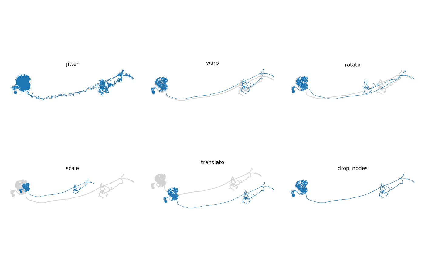
A few things to note from the panels above:

jitter roughens every point independently; warp bends the whole arbor smoothly (nearby points move together). Both preserve topology.
rotate and scale act about the centroid, so the neuron stays put; here we constrained the rotation to the z-axis and used a shrink range so the effect is visible.
translate relocates the whole neuron - the augmentation for models that are not translation-invariant.
drop_nodes thins a skeleton while keeping it connected: branch points and the root are never dropped and children reconnect through the gap, so the branching structure survives.

Note

drop_nodes supports TreeNeuron and Dotprops but not MeshNeuron (deleting vertices tears the surface - convert to skeleton/dotprops first). For skeletons, connectors on a dropped node are reattached to the nearest surviving ancestor, so none are left dangling.

Composing a pipeline: `augment_neuron`#

Rather than chaining these by hand, navis.ml.augment_neuron runs them in a sensible order - topology first, smooth deformation before the rigid transforms, and independent noise last:

graph LR
    D["drop"] --> W["warp"] --> R["rotate"] --> S["scale"] --> T["translate"] --> J["jitter"];

Each argument is None to skip that step, its primary value to run it with defaults, or a dict for full control.

variants = [
    navis.ml.augment_neuron(
        n, drop=0.1, warp=0.03, rotate=True, scale=(0.8, 1.25), jitter=0.01,
        random_state=seed,
    )
    for seed in range(5)
]

fig, axes = plt.subplots(1, 5, figsize=(18, 4))
navis.plot2d(n, method="2d", view=("x", "-z"), ax=axes[0], color="k", lw=0.7)
axes[0].set_title("original")
for ax, (i, v) in zip(axes[1:], enumerate(variants[:4])):
    navis.plot2d(v, method="2d", view=("x", "-z"), ax=ax, color="C0", lw=0.7)
    ax.set_title(f"augmented #{i}")
for ax in axes:
    ax.set_axis_off()
plt.tight_layout()

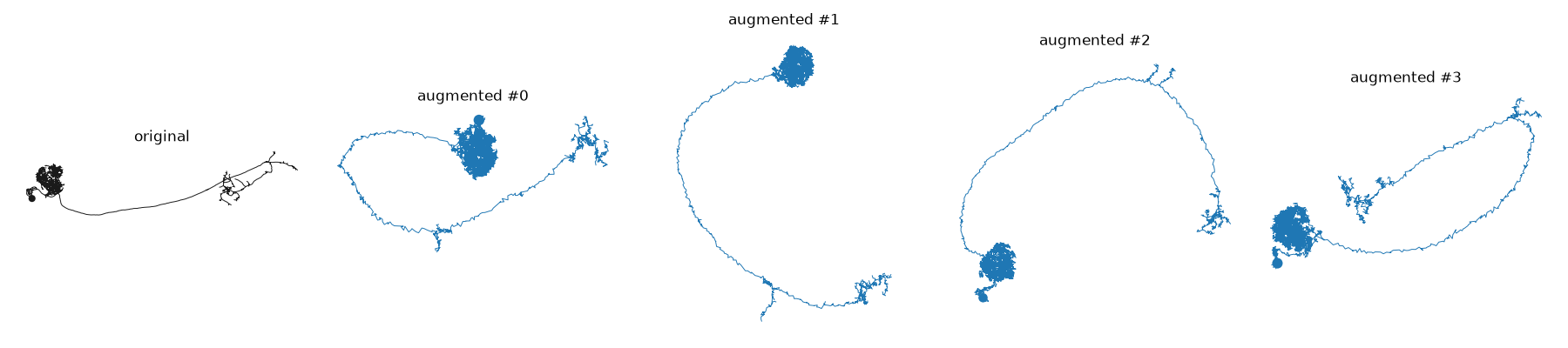
The whole pipeline is driven by a single random_state, so it is fully reproducible - same seed, same output:

a = navis.ml.augment_neuron(n, drop=0.1, rotate=True, jitter=0.02, random_state=0)
b = navis.ml.augment_neuron(n, drop=0.1, rotate=True, jitter=0.02, random_state=0)
print("reproducible:", np.array_equal(
    a.nodes[["x", "y", "z"]].values, b.nodes[["x", "y", "z"]].values
))

Out:

reproducible: True

Pass a dict to a step for finer control - e.g. constrain the rotation:

out = navis.ml.augment_neuron(
    n, rotate={"axis": "z", "max_angle": 15}, scale=(0.9, 1.1), random_state=0
)

Augmenting a whole population#

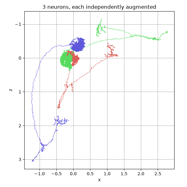
A NeuronList is augmented element-wise, each neuron getting an independent draw. This is exactly what you want when generating a batch of training examples:

nl = navis.ml.normalize_neuron(navis.example_neurons(3, kind="skeleton"))
aug = navis.ml.augment_neuron(nl, rotate=True, warp=0.03, jitter=0.01, random_state=0)

fig, ax = plt.subplots(figsize=(6, 6))
navis.plot2d(aug, method="2d", view=("x", "-z"), ax=ax, lw=0.6)
ax.set_title("3 neurons, each independently augmented")
plt.tight_layout()

Important

The Size units column above is why we normalized first: on a unit-RMS neuron a jitter sigma of ~0.01-0.05 is a gentle perturbation, but on a raw neuron in nanometers you would instead use something on the order of the node spacing.

A full training-input pipeline#

Chaining the three tutorials together, generating an augmented, fixed-size batch from raw neurons looks like this:

nl = navis.example_neurons(3, kind="skeleton")

def make_example(neuron, seed):
    norm = navis.ml.normalize_neuron(neuron)                 # 1. canonical pose
    aug = navis.ml.augment_neuron(                           # 2. perturb
        norm, rotate=True, warp=0.03, jitter=0.01, drop=0.1, random_state=seed
    )
    return navis.ml.sample_cable(                            # 3. fixed-size cloud
        aug, n_points=1024, random_state=seed
    )[["x", "y", "z"]].values

batch = np.stack([make_example(nrn, seed=0) for nrn in nl])
print("augmented model-input batch:", batch.shape)           # (n_neurons, 1024, 3)

Out:

augmented model-input batch: (3, 1024, 3)

What's next#

Normalizing Neurons - the canonical-pose step.
From Neurons to Model Inputs - sampling & chunking.

See the Machine Learning API reference for the full list of functions.

Total running time of the script: ( 0 minutes 3.163 seconds)

Download Python source code: tutorial_ml_02_augment.py

Download Jupyter notebook: tutorial_ml_02_augment.ipynb

Gallery generated by mkdocs-gallery

Augmenting Neurons#

The individual augmentations#

Composing a pipeline: augment_neuron#

Augmenting a whole population#

A full training-input pipeline#

What's next#

Composing a pipeline: `augment_neuron`#