Note
Click here to download the full example code
Transformations#
Move neurons between brain templates and mirror them across the midline.
As of version 0.5.0, NAVis can transform and mirror spatial data such as neurons. The functionality splits into high-level functions (which most users want) and the low-level building blocks. NAVis supports several transform types, each backed by a class you can also construct yourself:
| Transform type | navis class | Built from |
|---|---|---|
| CMTK warp | navis.transforms.CMTKtransform | a CMTK registration |
| Hdf5 deformation field | navis.transforms.H5transform | an HDF5 deformation field |
| Elastix | navis.transforms.ElastixTransform | an elastix transformation file |
| landmark thin-plate spline | navis.transforms.TPStransform | landmark correspondences |
| affine | navis.transforms.AffineTransform | a 4x4 matrix |
flybrains#
NAVis provides the machinery but ships no transforms of its own. Here we use flybrains, which registers a suite of Drosophila transforms directly with NAVis. Registering your own is covered further down.
Requires flybrains
This tutorial needs flybrains installed and its bridging registrations downloaded. Follow the flybrains instructions - including the data-download step - before running the code below.
import flybrains
Importing flybrains automatically registers the transforms with NAVis. This in turn allows NAVis to plot a sequence of bridging transformations to map between any connected template spaces.
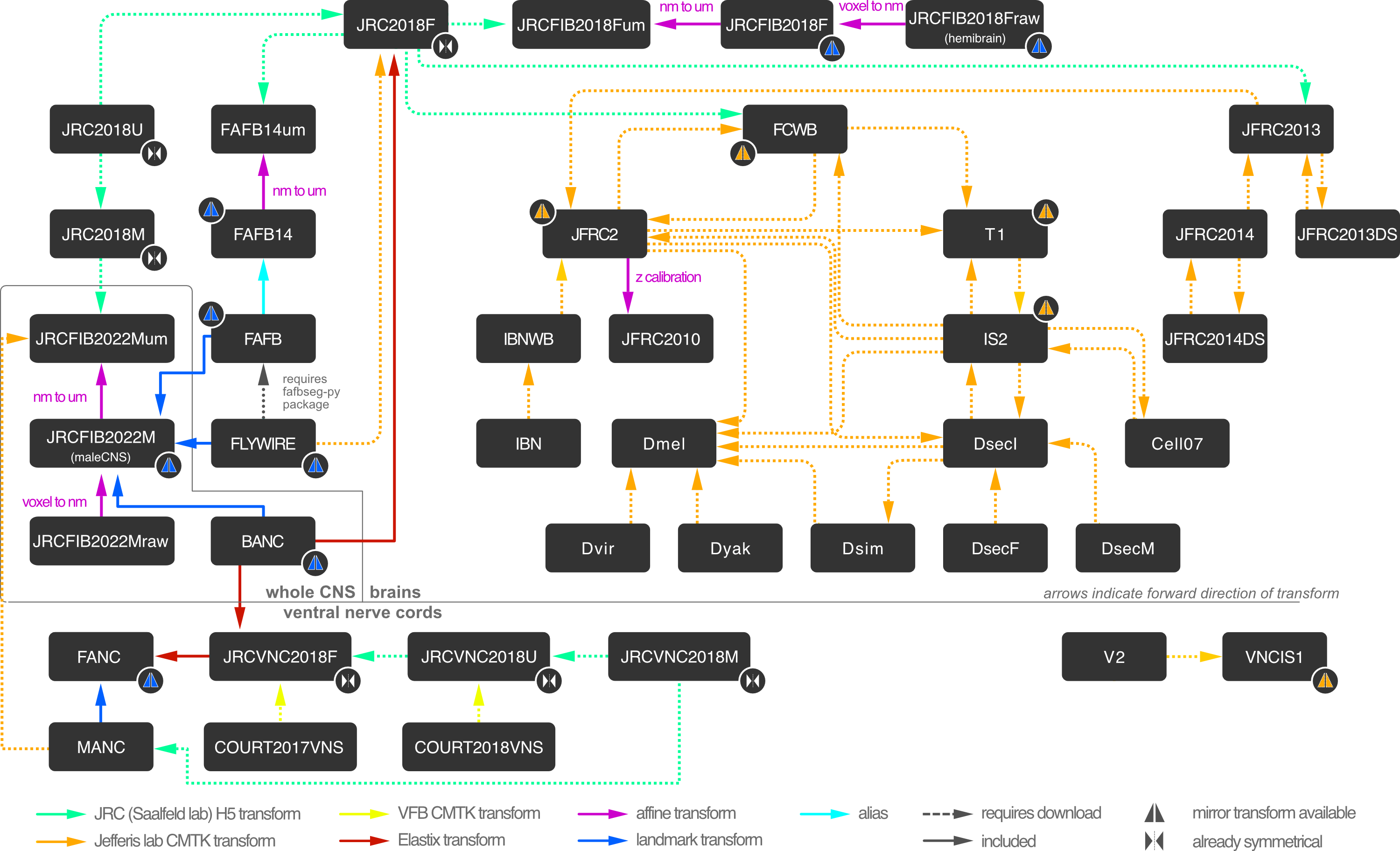
In addition to those bridging transforms, flybrains also contains mirror registrations (we will cover those later), meta data and meshes for the template brains:
# This is the Janelia "hemibrain" template brain
print(flybrains.JRCFIB2018F)
Out:
Template brain
--------------
Name: JRCFIB2018F
Short Name: JRCFIB2018F
Type: None
Sex:  F
Dimensions: 34432 x 39552 x 41408 voxels
Voxel size:
  x = 8 nanometers
  y = 8 nanometers
  z = 8 nanometers
Bounding box (nanometers):
  x = 0, y = 0, z = 0,
  x = 275456, y = 316416, z = 331264,
Description: Nanometer-calibrated version of Janelia FIB hemibrain dataset.
DOI: https://doi.org/10.1101/2020.01.21.911859
import navis
import matplotlib.pyplot as plt

# This is the hemibrain neuropil surface mesh
fig, ax = navis.plot2d(flybrains.JRCFIB2018F, view=("x", "-z"))
plt.tight_layout()
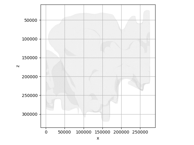
You can check the registered transforms like so:
navis.transforms.registry.summary()

# !!! note
#     The documentation is built in an environment with a minimal number of transforms registered. If you have installed
#     and imported `flybrains`, you should see a lot more than what is shown above.
Using xform_brain#
For high-level transforming, you will want to use navis.xform_brain. This function takes a source and target argument and tries to find a bridging sequence that gets you to where you want. Let's try it out:
Info
Incidentally, the example neurons that NAVis ships with are from the Janelia hemibrain project and are therefore in JRCFIB2018raw space ("raw" means uncalibrated voxel space which is 8x8x8nm for this dataset). We will be using those but there is nothing stopping you from using the NAVis interface with neuPrint (the tutorials on interfaces) to fetch your favourite hemibrain neurons and transform those.
# Load the example hemibrain neurons (JRCFIB2018raw space)
nl = navis.example_neurons()
nl
fig, ax = navis.plot2d([nl, flybrains.JRCFIB2018Fraw], view=("x", "-z"))
plt.tight_layout()
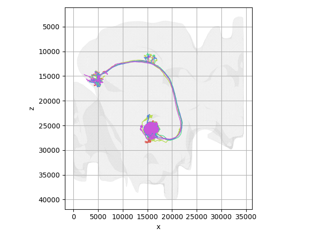
Let's say we want these neurons in JRC2018F template space. Before running the transform, it's worth tracing the path navis.xform_brain will take through the bridging graph:
What is JRC2018F?
JRC2018F is a standard brain made from averaging over multiple fly brains. See Bogovic et al., 2020 for details.
graph LR
    A["JRCFIB2018Fraw"] -->|"affine: voxels to nm"| B["nanometers"];
    B -->|"affine: nm to um"| C["JRCFIB2018Fum"];
    C -->|"Hdf5 (Saalfeld lab)"| D["JRC2018F"];
Two affine steps take us from raw voxels to micrometers, then a Saalfeld-lab Hdf5 transform maps JRCFIB2018Fum onto JRC2018F. Arrows show each transform's forward direction, but NAVis can invert any of them to traverse the graph in reverse.
xf = navis.xform_brain(nl, source="JRCFIB2018Fraw", target="JRC2018F")
Out:
Transform path: JRCFIB2018Fraw -> JRCFIB2018F -> JRCFIB2018Fum -> JRC2018F
Let's see if it worked:
Plot the transformed neurons and the JRC2018F template brain
fig, ax = navis.plot2d([xf, flybrains.JRC2018F], color="r", view=("x", "-y"))
plt.tight_layout()
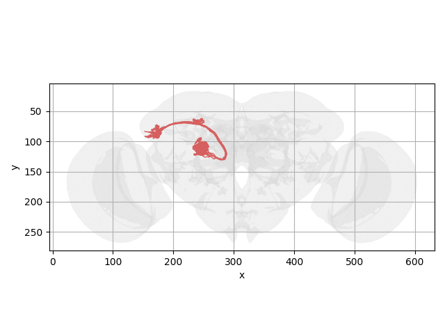
Take a look at navis.xform_brain's parameters to fine-tune the transform.
Using mirror_brain#
navis.mirror_brain mirrors neurons across the midline - e.g. from the left to the right side of a brain.
How mirroring works
Mirroring happens in two steps:
- Reflect coordinates about the midpoint of the mirror axis (an affine transformation).
- Optionally apply a warping transform to compensate for left/right asymmetries.
Step 1 needs the length of the mirror axis, so - as with registered transforms - NAVis must have meta data about the template space (its bounding box) available.
Step 2 is optional: JRC2018F and JRC2018U are averaged from many brains and are already mirror symmetrical, so they need no warping. flybrains does ship mirror transforms for others, e.g. FCWB, VNCIS1 or JFRC2.
Since our neurons are already in JRC2018F space, let's try mirroring them:
mirrored = navis.mirror_brain(xf, template="JRC2018F")
fig, ax = navis.plot2d(
    [xf, mirrored, flybrains.JRC2018F], color=["r"] * 5 + ["g"] * 5, view=("x", "-y")
)
plt.tight_layout()
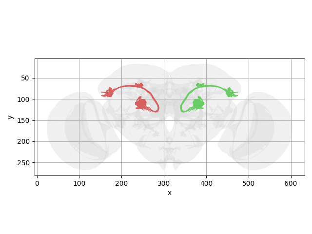
As noted above, this only works if the template is registered with NAVis and contains its bounding box. If you only have the bounding box but no template brain, check out the lower-level function navis.transforms.mirror.
Low-level functions#
Adding your own transforms#
To add your own transform, pick the matching class from the table at the top of this page and construct it directly. Here we build a thin-plate spline transform with navis.transforms.TPStransform. If you look at the bridging graph again, you might note the "FAFB14" template brain: it stands for "Full Adult Fly Brain" (the 14 is a version number for the alignment). We will use landmarks to generate a mapping between this 14th and the previous 13th iteration.
First we will grab the landmarks from the Saalfeld's lab elm repository:
import pandas as pd

# These landmarks map between FAFB (v14 and v13) and a light level template
# We will use only the v13 and v14 landmarks
landmarks_v14 = pd.read_csv(
    "https://github.com/saalfeldlab/elm/raw/master/lm-em-landmarks_v14.csv", header=None
)
landmarks_v13 = pd.read_csv(
    "https://github.com/saalfeldlab/elm/raw/master/lm-em-landmarks_v13.csv", header=None
)

# Name the columns
landmarks_v14.columns = landmarks_v13.columns = [
    "label",
    "use",
    "lm_x",
    "lm_y",
    "lm_z",
    "fafb_x",
    "fafb_y",
    "fafb_z",
]

landmarks_v13.head()
Now we can use those landmarks to generate a thin plate spline transform:
from navis.transforms.thinplate import TPStransform

tr = TPStransform(
    landmarks_source=landmarks_v14[["fafb_x", "fafb_y", "fafb_z"]].values,
    landmarks_target=landmarks_v13[["fafb_x", "fafb_y", "fafb_z"]].values,
)
# note: navis.transforms.MovingLeastSquaresTransform has similar properties
The transform has a method that we can use to transform points but first we need some data in FAFB14 space:
# Transform our neurons into FAFB 14 space
xf_fafb14 = navis.xform_brain(nl, source="JRCFIB2018Fraw", target="FAFB14")
Out:
Transform path: JRCFIB2018Fraw -> JRCFIB2018F -> JRCFIB2018Fum -> JRC2018F -> FAFBum = FAFB14um -> FAFB14
Now let's see if we can use the v14v13 transform:
# Transform the nodes of the first two neurons
pts_v14 = xf_fafb14[:2].nodes[["x", "y", "z"]].values
pts_v13 = tr.xform(pts_v14)
Out:
/opt/hostedtoolcache/Python/3.11.15/x64/lib/python3.11/site-packages/morphops/tps.py:157: DeprecationWarning: `row_stack` alias is deprecated. Use `np.vstack` directly.
  Y_0 = np.row_stack((Y, np.zeros((n_coords+1,n_coords))))
Quick check how the v14 and v13 coordinates compare:
# Original in black, transformed in red
fig, ax = navis.plot2d(pts_v14, scatter_kws=dict(c="k"), view=("x", "-y"))
_ = navis.plot2d(pts_v13, scatter_kws=dict(c="r"), ax=ax, view=("x", "-y"))
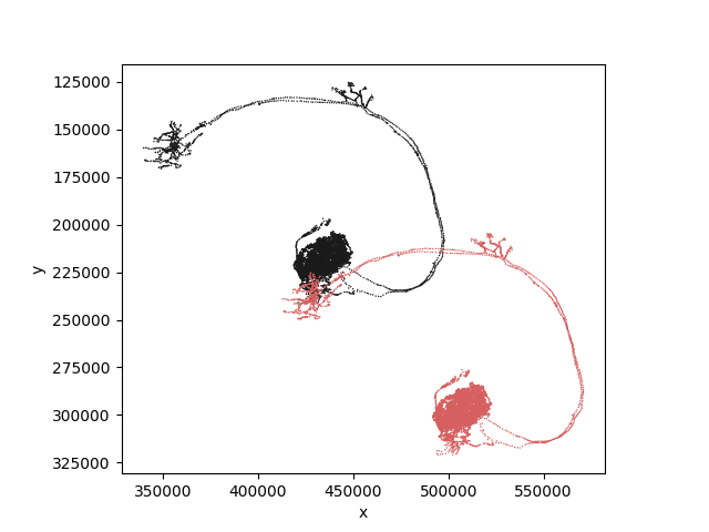
Next, we will register this new transform with NAVis so we can use it with the higher-level functions:
# Register the transform
navis.transforms.registry.register_transform(
    tr, source="FAFB14", target="FAFB13", transform_type="bridging"
)
Now that's done we can use FAFB13 with navis.xform_brain:
# Transform our neurons into FAFB 14 space
xf_fafb13 = navis.xform_brain(xf_fafb14, source="FAFB14", target="FAFB13")
Out:
Transform path: FAFB14 -> FAFB13
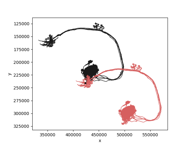
fig, ax = navis.plot2d(xf_fafb14, c='k', view=("x", "-y"))
_ = navis.plot2d(xf_fafb13, c='r', ax=ax)
Registering Template Brains#
For completeness, let's also have a quick look at registering additional template brains.
Template brains are represented in navis as navis.transforms.templates.TemplateBrain and there is currently no canonical way of constructing them: you can associate as much or as little data with them as you like. However, for them to be useful they should have a name, a label and a boundingbox property.
Minimally, you could do something like this:
# Construct template brain from base class
my_brain = navis.transforms.templates.TemplateBrain(
    name="My template brain",
    label="my_brain",
    boundingbox=[[0, 100], [0, 100], [0, 100]],
)

# Register with navis
navis.transforms.registry.register_templatebrain(my_brain)

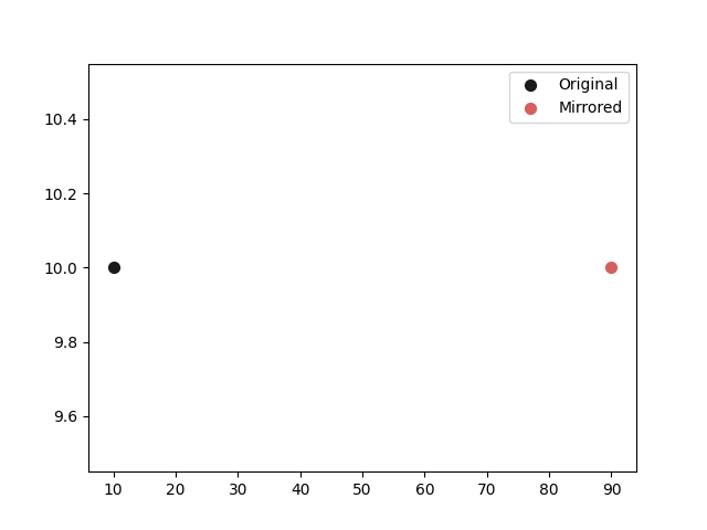
# Now you can use it with mirror_brain:
import numpy as np

pts = np.array([[10, 10, 10]])
pts_mirrored = navis.mirror_brain(pts, template="my_brain")

# Plot the points
fig, ax = plt.subplots()
ax.scatter(pts[:, 0], pts[:, 1], c="k", alpha=1, s=50, label="Original")
ax.scatter(
    pts_mirrored[:, 0], pts_mirrored[:, 1], c="r", alpha=1, s=50, label="Mirrored"
)
ax.legend()
Out:
<matplotlib.legend.Legend object at 0x7fa27df33e50>
While this is a working solution, it's not very pretty: for example, my_brain does have the default docstring and no fancy string representation (e.g. for print(my_brain)). I highly recommend you take a look at how flybrains constructs and packages the templates.
Affines in Neuroglancer#
Neuroglancer can attach an affine transform to each data source, which is the quickest way to overlay data from two affine-related spaces without re-generating anything. Feeding it a NAVis matrix is trivial once you know the conventions - so let's nail those down.
Every data source in a layer's Source tab carries such a matrix - 3x4 for ordinary 3D data - plus a scale for each source and output dimension:
source x8nm | source y8nm | source z40nm | translation | |
|---|---|---|---|---|
output x 8nm | 1 | 0 | 0 | 0 |
output y 8nm | 0 | 1 | 0 | 0 |
output z 40nm | 0 | 0 | 1 | 0 |
Three rules are all you need:
- Rows are output dimensions, columns are source dimensions, plus a trailing translation column. That is exactly the layout of a NAVis
4x4matrix minus its[0, 0, 0, 1]bottom row - no transposing required. - The
3x3block acts on physical coordinates. Neuroglancer multiplies each coefficient bysource scale / output scaleinternally, so what you type is scale-free: an identity block means "leave the data where it is", whether the source voxels are 8nm or 8µm. Never hand-compensate for voxel size here. - The translation column is in output units, not nanometers. With output dimensions of
8nm, a translation of1moves the layer by 8nm - so divide your offsets by the output scale.
graph LR
    A["source coords<br>(e.g. voxels)"] -->|"× source scale"| B["physical space"];
    B -->|"3×3 block"| C["physical space"];
    C -->|"÷ output scale"| D["output coords"];
    D -->|"+ translation"| E["global position"];
The translation column is where everyone gets burned
Rule 3 cuts both ways: editing an output dimension's scale afterwards leaves your translation number untouched but changes what it means. A translation of 73341 is 73µm while the output dimension reads 1nm and 587µm once you switch it to 8nm - the linear block, in contrast, is immune. When in doubt, set the output dimensions to 1nm and paste nanometers verbatim.
Let's convert the FAFB14 FAFB13 thin-plate spline from earlier. TPS (and moving least squares) transforms expose their affine component directly:
tr.matrix_affine
Out:
array([[ 9.99919159e-01, -8.02765083e-04, -9.69556317e-05,
         7.33413307e+04],
       [ 4.26179745e-04,  1.00077606e+00, -2.05564634e-04,
         7.88998986e+04],
       [-9.65910992e-06, -1.85687246e-06,  8.74965776e-01,
         7.63124316e+00],
       [ 0.00000000e+00,  0.00000000e+00,  0.00000000e+00,
         1.00000000e+00]])
The conversion is then a two-liner: drop the bottom row, and divide the translation by the output scale.
def to_neuroglancer(matrix, output_scale=(1, 1, 1)):
    """Convert a navis affine matrix into a neuroglancer transform.

    Parameters
    ----------
    matrix :        (4, 4) array
                    Affine matrix mapping nanometers to nanometers.
    output_scale :  tuple
                    Scale of neuroglancer's output dimensions, in nanometers.

    Returns
    -------
    dict
                    Drop this into a layer's 'source' in the JSON state.

    """
    m = np.asarray(matrix, dtype=float)[:3, :4].copy()  # drop the [0, 0, 0, 1] row
    m[:, 3] /= np.asarray(output_scale, dtype=float)  # translation into output units
    return {
        "matrix": m.tolist(),
        "outputDimensions": {
            dim: [float(s), "nm"] for dim, s in zip("xyz", output_scale)
        },
    }


# The public FAFB v14 EM layer has 8 x 8 x 40 nm voxels
transform = to_neuroglancer(tr.matrix_affine, output_scale=(8, 8, 40))

np.round(transform["matrix"], 6)
Out:
array([[ 9.99919000e-01, -8.03000000e-04, -9.70000000e-05,
         9.16766634e+03],
       [ 4.26000000e-04,  1.00077600e+00, -2.06000000e-04,
         9.86248732e+03],
       [-1.00000000e-05, -2.00000000e-06,  8.74966000e-01,
         1.90781000e-01]])
Note how the translation shrank from ~73,000 (nanometers) to ~9,200 (multiples of the 8nm output dimension).
My transform isn't in nanometers
Plenty of template spaces are calibrated in microns (JRC2018F, FCWB, ... - anything ending in um), and a matrix inherits the units of the landmarks it was built from. Rescale it before converting:
um_to_nm = np.diag([1e3, 1e3, 1e3, 1])
matrix_nm = um_to_nm @ matrix_um @ np.linalg.inv(um_to_nm)
The 3x3 block comes out unchanged (it is unit-free) while the translation is scaled by 1,000. Mixed units - e.g. nanometers in, microns out - work the same way: pre-multiply with the output conversion, post-multiply with the inverse of the input conversion.
Hit the {} button ("Edit JSON state") in Neuroglancer's top right corner and give the layer's source the transform we just built:
{
  "type": "image",
  "name": "FAFB v14 in v13 space",
  "source": {
    "url": "precomputed://gs://neuroglancer-fafb-data/fafb_v14/fafb_v14_clahe",
    "transform": {
      "matrix": [
        [0.999919, -0.000803, -0.000097, 9167.666339],
        [0.000426,  1.000776, -0.000206, 9862.487323],
        [-0.00001, -0.000002,  0.874966,    0.190781]
      ],
      "outputDimensions": {"x": [8, "nm"], "y": [8, "nm"], "z": [40, "nm"]}
    }
  }
}
The same numbers can of course be typed straight into the matrix widget in the Source tab - the JSON route just spares you 12 rounds of click-and-tab.
Source dimensions that aren't x/y/z
Columns follow the source dimensions in the order the widget lists them and rows follow the output dimensions. precomputed sources are x/y/z, but n5, zarr & co. often come as z/y/x or even d0/d1/d2. In that case permute the matrix to match, e.g. matrix[np.ix_([2, 1, 0], [2, 1, 0, 3])] to flip x/y/z z/y/x. Renaming the output dimensions in the widget is an easier way to permute rows only.
Before hunting for the layer in the browser, we can check our work by reproducing what Neuroglancer will do with those numbers:
def apply_like_neuroglancer(transform, points, source_scale):
    """Apply a neuroglancer transform the way neuroglancer does. Nanometers in, nanometers out."""
    m = np.asarray(transform["matrix"], dtype=float)
    source_scale = np.asarray(source_scale, dtype=float)
    output_scale = np.array([s for s, _ in transform["outputDimensions"].values()])

    # Neuroglancer rescales the 3x3 block by source/output scale but leaves the translation alone
    linear = m[:, :3] * (source_scale / output_scale[:, None])

    return ((points / source_scale) @ linear.T + m[:, 3]) * output_scale


# The affine part of the transform, applied by navis
expected = pts_v14 @ tr.matrix_affine[:3, :3].T + tr.matrix_affine[:3, 3]

# The same points, run through the neuroglancer transform
actual = apply_like_neuroglancer(transform, pts_v14, source_scale=(8, 8, 40))

print(f"Largest deviation: {np.abs(actual - expected).max():.2e} nm")
Out:
Largest deviation: 5.82e-11 nm
Fitting an affine to a warping transform#
.matrix_affine only exists for thin-plate spline and moving least squares transforms. For a CMTK, Hdf5 or elastix registration - or whenever you want the best affine approximation rather than the affine component that happens to fall out of a spline fit - fit one yourself to a cloud of transformed points:
# Sample points across the source template's bounding box and transform them
rng = np.random.default_rng(0)
bbox = np.asarray(flybrains.FAFB14.boundingbox).reshape(3, 2)
pts = rng.uniform(bbox[:, 0], bbox[:, 1], size=(1_000, 3))
pts_xf = tr.xform(pts)  # this could be any navis transform

# Least-squares fit of an affine to the point correspondences
solution, *_ = np.linalg.lstsq(
    np.hstack((pts, np.ones((len(pts), 1)))), pts_xf, rcond=None
)
matrix_fitted = np.eye(4)
matrix_fitted[:3] = solution.T

np.round(matrix_fitted, 6)
Out:
array([[ 9.99871000e-01, -5.70000000e-04, -1.92000000e-04,
         7.32605517e+04],
       [ 2.48000000e-04,  1.00021500e+00, -2.36000000e-04,
         7.91993431e+04],
       [ 0.00000000e+00, -1.00000000e-05,  8.74956000e-01,
        -3.27375000e-01],
       [ 0.00000000e+00,  0.00000000e+00,  0.00000000e+00,
         1.00000000e+00]])
How much do we lose by dropping the non-linear part? Let's compare both affines against the full transform:
def residuals(matrix):
    return np.linalg.norm(pts @ matrix[:3, :3].T + matrix[:3, 3] - pts_xf, axis=1)


print(f"TPS affine component: {np.median(residuals(tr.matrix_affine)):>4.0f} nm median error")
print(f"Fitted affine:        {np.median(residuals(matrix_fitted)):>4.0f} nm median error")
Out:
TPS affine component:  108 nm median error
Fitted affine:          49 nm median error
Both land within a fraction of a micron here because FAFB14 FAFB13 is almost rigid. Warps between different brains (e.g. JRC2018F FAFB14) deform much more and no affine will do them justice - use navis.xform_brain and upload the transformed data instead.
Which direction?
A layer's transform maps that layer's data into the viewer's space. So if the layer holds FAFB14 data and you want to see it in FAFB13 space, you need the FAFB14 FAFB13 matrix, as above. Got the transform the wrong way around? np.linalg.inv(matrix) fixes it.
Acknowledgments#
Much of the transform module is modelled after functions written by Greg Jefferis for the natverse. Likewise, flybrains is a port of data collected by Greg Jefferis for nat.flybrains and nat.jrcbrains.
Total running time of the script: ( 0 minutes 4.272 seconds)
Download Python source code: tutorial_misc_01_transforms.py
Download Jupyter notebook: tutorial_misc_01_transforms.ipynb