Note
Click here to download the full example code
Cortical Neurons#
Recreate a published figure of cortical GABAergic neurons arranged by soma depth.
In this exercise we will visualize morphological data from "Integrated Morphoelectric and Transcriptomic Classification of Cortical GABAergic Cells" by Gouwens, Sorensen et al., Cell (2020). Specifically, we will re-create a plot similar to their Figure 4A.

The pipeline in a nutshell:
graph LR
    A[Load neurons<br>from BIL] --> B[Align by<br>soma depth];
    B --> C[Layered<br>plot];
    C --> D[Depth KDE];
Needs network access
This tutorial downloads reconstructions from the Brain Image Library (BIL) at runtime, so it needs an internet connection.
For brevity, we will use some fixed cell IDs and properties from the dataset. These were taken from the 20200711_patchseq_metadata_mouse.csv file provided alongside the supplementary material of the paper:
# The cell IDs we will use (it's the first 5 in the meta data file)
ids = [601506507, 601790961, 601803754, 601808698, 601810307]

# The normalized soma depths for these cells (also from the meta data file)
soma_depths = [0.36101451, 0.62182935, 0.16423996, 0.48303029, 0.2956563]
Part I: Loading and Aligning Neurons#
First we need to load the neurons. These reconstructions live in the Brain Image Library (BIL) and NAVis ships an interface for it.
BIL stores this collection as one small dataset per cell, each indexed by the very cell ID we already have. So we can look up the dataset for each of our cells, then grab the transformed SWC file from it:
import navis
import navis.interfaces.brain_image_library as bil

# Look up the BIL dataset for each of our cells
datasets = [bil.query("specimen", "localid", str(i))[0] for i in ids]

# Load the transformed skeletons (each dataset also contains a raw SWC and a marker file)
nl = bil.get_neurons(datasets, pattern="*_transformed.swc")

# The neurons come back in the order we asked for them, so we can just re-attach the cell IDs
nl.set_neuron_attributes(ids, name="id")
nl.set_neuron_attributes([str(i) for i in ids], name="name")
To make our lives a bit easier, we will attach the soma depth to the neurons as metadata:
nl.set_neuron_attributes(
    soma_depths,
    name="cell_soma_normalized_depth",
    register=True
    )

nl
Next, we align the neurons by soma depth. The normalized cell_soma_normalized_depth maps onto a physical range of 0 to 922.586 microns. Let's work through one neuron first:
# Grab one of the neurons
n = nl[0]

# This is the normalized soma depth:
print(f"Normalized soma depth: {n.cell_soma_normalized_depth}")
Out:
Normalized soma depth: 0.36101451
Why we position from the bottom
The physical soma depth is just the normalized depth times the total cortical depth (922.586 microns). We position from the bottom - so 922.586 is at the surface and 0 at the bottom - because matplotlib's origin sits in the bottom-left corner, which keeps the plotting math simple.
phys_y = (1 - n.cell_soma_normalized_depth) * 922.5861720311
print(f"Physical soma depth: {phys_y}")

# Current soma
print(f"Current soma coordinates: {n.soma_pos[0]}")
Out:
Physical soma depth: 589.5191772025167
Current soma coordinates: [382.803   433.69104 118.07384]
We will now offset the neuron such that the soma is at (0, 589.519, 0):
offset = [0, phys_y, 0] - n.soma_pos[0]
offset
Out:
array([-382.80300903, 155.82813716, -118.07383728])
Moving or scaling neurons in NAVis is straightforward: adding, subtracting, multiplying or dividing a neuron by a number or an [x, y, z] vector changes its coordinates:
# Move the neuron to the new centered position
n += offset

# Check that the soma is now in the correct position
n.soma_pos[0]
Out:
array([ 0. , 589.5191772, 0. ])
That looks good! Let's do it for all neurons:
for n in nl:
    phys_y = (1 - n.cell_soma_normalized_depth) * 922.5861720311
    offset = [0, phys_y, 0] - n.soma_pos[0]
    n += offset
Check that all soma positions are correct:
nl.soma_pos.reshape(-1, 3)
Out:
array([[  0.        , 589.5191772 ,   0.        ],
       [  0.        , 348.89501236,   0.        ],
       [  0.        , 771.06065604,   0.        ],
       [  0.        , 476.9491058 ,   0.        ],
       [  0.        , 649.81775798,   0.        ]])
Part II: Plotting#
Now that the neurons are loaded and aligned, let's recreate a plot similar to Figure 4A.
The SWC files carry a label column encoding each node's compartment, which we map to colors:
compartment_palette = {
    1: color,       # (1)!
    2: axon_color,  # (2)!
    3: color,       # (3)!
}
1= soma2= axon3= dendrites
We also draw the cortical layer boundaries - the top bound of each layer, in microns from the surface:
| Layer | Top bound (µm) |
|---|---|
| L1 | 0 |
| L2/3 | 115.11 |
| L4 | 333.47 |
| L5 | 453.62 |
| L6 | 687.65 |
| L6b | 883.13 |
The helper below wraps it all up:
def plot_neurons(to_plot, color="purple", axon_color="magenta", offset=500):
    """Plot all neurons of a given transcriptomic type.

    Parameters
    ----------
    neurons : NeuronList
        The aligned neurons to plot.
    color : str
        The color of the dendrites.
    axon_color : str
        The color of the axon.
    offset : int
        The offset between neurons along the x-axis.

    Returns
    -------
    fig, ax
        The matplotlib figure and axis.

    """
    # Offset the neurons along the x-axis so that they don't overlap
    to_plot = [n + [offset * i, 0, 0] for i, n in enumerate(to_plot)]

    # Map each compartment `label` (1=soma, 2=axon, 3=dendrites) to a color:
    compartment_palette = {1: color, 2: axon_color, 3: color}

    # Plot the neuron
    fig, ax = navis.plot2d(
        to_plot,
        radius=False,
        lw=1.5,
        soma=dict(
            fc="black",  # soma fill color
            ec="white",  # highlight the soma with a white outline
            radius=10,   # override the default soma radius
        ),
        color_by="label",  # color by `label` column in node table
        palette=compartment_palette,
        figsize=(
            len(to_plot) * 2,
            10,
        ),  # scale the figure size with the number of neurons
        method="2d",
    )

    # Add the layer boundaries (top bound for each layer in microns)
    layer_bounds = {
        "L1": 0,
        "L2/3": 115.1112491335,
        "L4": 333.4658190171,
        "L5": 453.6227158132,
        "L6": 687.6482650269,
        "L6b": 883.1308910545,
    }

    for layer, y in layer_bounds.items():
        y = 922.5861720311 - y  # flip the y-axis
        # Add a dashed line
        ax.axhline(y, color="gray", ls="--", lw=1)
        # Add the layer name
        ax.text(-300, y - 25, layer, color="gray", va="center", size=10)
    # Add the bottom bound
    ax.axhline(0, color="gray", ls="--", lw=1)

    # Set the axis y limits according to the layers
    ax.set_ylim(-10, 930)

    # Hide axes
    ax.axis("off")

    return fig, ax


fig, ax = plot_neurons(nl)
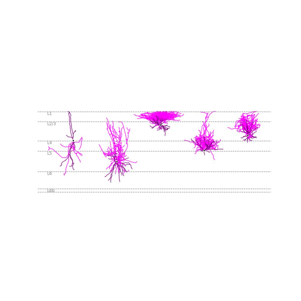
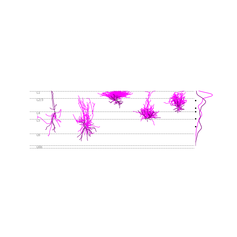
That looks close enough. The last bit is to add the little KDE plots for the depth-distribution of cable length!
We're going to be cheap here and simply generate a histogram over the node positions. To make this representative, we should make sure that the number of nodes per unit of cable is homogeneous across neurons. For that we will resample the neurons:
print(
    f"Sampling rate (nodes per micron of cable) before resampling: {nl.sampling_resolution.mean():.2f}"
)

# Resample to 2 nodes per micron
resampled = navis.resample_skeleton(
    nl,
    resample_to=0.5,
    map_columns="label",  # make sure label column is carried over
)

print(
    f"Sampling rate (nodes per micron of cable) after resampling: {resampled.sampling_resolution.mean():.2f}"
)
Out:
Sampling rate (nodes per micron of cable) before resampling: 1.57
Sampling rate (nodes per micron of cable) after resampling: 0.50
Get the combined nodes table:
nodes = resampled.nodes
nodes.head()
Now we can plot the distribution of cable lengths for our neurons:
import seaborn as sns
from mpl_toolkits.axes_grid1 import make_axes_locatable

# Plot the neurons again, re-using the function we defined above
fig, ax = plot_neurons(nl)

# Add a new axis to the right of the main plot
divider = make_axes_locatable(ax)
ax_hist = divider.append_axes("right", size=0.75, pad=0.05)

# Add histograms
# For axon:
sns.kdeplot(
    data=nodes[nodes.label == 2], y="y", ax=ax_hist, color="magenta", linewidth=1.5
)
# For the rest:
sns.kdeplot(
    data=nodes[nodes.label != 2], y="y", ax=ax_hist, color="purple", linewidth=1.5
)

# Add soma positions
soma_pos = nl.soma_pos.reshape(-1, 3)
ax_hist.scatter([0] * len(soma_pos), soma_pos[:, 1], color="black", s=10, clip_on=False)

# Set same axis limits as the main plot
ax_hist.set_ylim(-10, 930)

# Hide axes
ax_hist.set_axis_off()
Acknowledgements#
We thank Staci Sorensen and Casey Schneider-Mizell from the Allen Institute for Brain Science for helping with extra information and data for this tutorial!
Total running time of the script: ( 0 minutes 8.898 seconds)
Download Python source code: tutorial_plotting_06_cortex.py
Download Jupyter notebook: tutorial_plotting_06_cortex.ipynb