Note
Click here to download the full example code
Analyzing Neuron Morphology#
Measure morphometrics — segment lengths, geodesic distances and branch angles.
Disclaimer: As you might imagine some properties can be gathered for all/most neuron types while others will only work on specific types. For example, topological properties such as cable length, branch points, etc. are easy to get for a skeleton (i.e. a TreeNeuron) but not for an image (i.e. a VoxelNeuron). Make sure to check the respective function's docstring for details!
Basic Properties#
NAVis provides some basic morphometrics as neuron properties. Others need to be computed using a specific function (e.g. navis.tortuosity) - mostly because they require/allow some parameters to be set.
With that in mind:
import navis
import matplotlib.pyplot as plt

import seaborn as sns

sns.set_color_codes("muted")
Accessing attributes for a single neuron:
# Load a single skeleton (i.e. a TreeNeuron)
n = navis.example_neurons(n=1, kind="skeleton")
print(f"This neuron has {n.cable_length} of cable")
Out:
This neuron has 266476.875 of cable
If your neuron has its units properties set, you can also combine those:
print(f"This neuron has {(n.cable_length * n.units).to('microns')} of cable")
Out:
This neuron has 2131.815185546875 micron of cable
Accessing the same properties via a navis.NeuronList will return an array:
nl = navis.example_neurons(kind="skeleton")
print(f"Cable lengths for neurons in this list:\n{nl.cable_length}")
Out:
Cable lengths for neurons in this list:
[266476.88 304332.66 274703.38 286522.47 291265.3 ]
navis.NeuronList.summary is a useful way to collect some of the basic parameters:
df = nl.summary()
df.head()
For MeshNeurons the available properties look different. For example, you can get its volume:
# Load a single MeshNeuron
m = navis.example_neurons(n=1, kind="mesh")
print(f"Neuron volume: {m.volume}")

# Again, we can use the `units` property to convert:
print(f"Neuron volume: {(m.volume * n.units **3).to('microns ** 3')}")
Out:
Neuron volume: 1291610825.1668386
Neuron volume: 661.3047424854216 micron ** 3
For topological properties, we need to convert to skeleton. The fastest way is to simply access the MeshNeuron's .skeleton property:
print(f"Mesh cable length: {m.skeleton.cable_length * m.units}")
Out:
Mesh cable length: 1351124.75 nanometer
Note
The above .skeleton property is simply an automatically generated TreeNeuron representation of the mesh. It uses sensible defaults but as said initially: it's good practice to create and check the skeleton yourself via navis.skeletonize.
Importantly, some NAVis functions (e.g. navis.segment_analysis, see below) that accept MeshNeurons as input, really use this skeleton representation under-the-hood.
The skeleton representation of the mesh lets us access many topological properties:
m.skeleton.n_leafs
Out:
156
m.skeleton.n_branches
Out:
122
The n_ prefix
You may have noticed the n_{property} pattern (e.g. n.n_leafs). It's generic: prefix any existing attribute with n_ and - assuming that property exists - NAVis returns its count.
m.n_vertices
Out:
6309
m.skeleton.n_nodes
Out:
1058
# Illustrate with a random property
m.my_counts = [1, 2, 3, 4, 5]
m.n_my_counts
Out:
5
Segment Analysis#
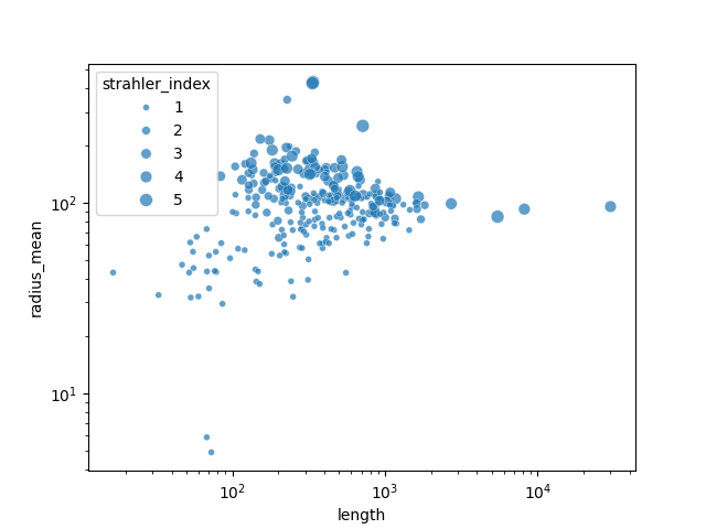
navis.segment_analysis is a great entry point for collecting a bunch of morphometrics for your neuron(s) of interest. It returns Strahler index, cable length, distance to root, radius and tortuosity for each linear segment:
sa = navis.segment_analysis(m)
sa.head()
# See if segment length correlates with radius
ax = sns.scatterplot(
    data=sa, x="length", y="radius_mean", size="strahler_index", alpha=0.7
)
ax.set_xscale("log")
ax.set_yscale("log")
Sholl Analysis#
-
Sholl analysis
A worked Sholl analysis lives in the MICrONS tutorial.
Branch, Path & Soma-Exit Angles#
NAVis can also measure the angles in a neuron's geometry:
| Function | Measures |
|---|---|
navis.branch_angles | angle between child branches at each branch point |
navis.path_angles | bend at each continuation (slab) node |
navis.root_angles | each segment's angle relative to the root direction |
navis.soma_exit_angles | angles between the neurites leaving the soma |
These are most informative for neurons with a clear dendritic/axonal layout such as vertebrate cortical cells. The example neurons we have used so far are insect neurons, so we instead pull a few mouse cortical reconstructions from the Brain Image Library (BIL).
Fetches remote data
The branch-angle examples below download a handful of reconstructions from the Brain Image Library, so this section needs an internet connection.
import pandas as pd

import navis.interfaces.brain_image_library as bil

# A handful of patch-seq mouse cortical cells (the same dataset as the "Cortical Neurons"
# plotting tutorial). These SWCs carry a `label` column: 1 = soma, 2 = axon, 3 = dendrite.
ids = [601506507, 601790961, 601803754]
datasets = [bil.query("specimen", "localid", str(i))[0] for i in ids]
cortical = bil.get_neurons(datasets, pattern="*_transformed.swc")

# The angle metrics are measured relative to the root, so root each neuron at its soma:
for cn in cortical:
    cn.reroot(cn.soma, inplace=True)

cortical
navis.branch_angles returns one row per branch point, so the result is effectively a distribution we can summarize or plot. Let's compute it per neuron and use the label column to split the branch angles by compartment (axon vs dendrite):
frames = []
for cn in cortical:
    b = navis.branch_angles(cn)
    # Map each branch point onto its compartment label (per-neuron, since node IDs
    # are only unique within a neuron)
    b["compartment"] = b.node_id.map(cn.nodes.set_index("node_id").label)
    frames.append(b)

ba = pd.concat(frames, ignore_index=True)
ba["compartment"] = ba.compartment.map({2: "axon", 3: "dendrite"})
ba.head()
Now we can compare the branch-angle distributions between axon and dendrite:
ax = sns.violinplot(
    data=ba.dropna(subset=["compartment"]),
    x="compartment",
    y="branch_angle",
    cut=0,
)
_ = ax.set_ylabel("branch angle (degrees)")
The other angle functions behave the same way. For instance, navis.soma_exit_angles gives the angles between the neurites leaving the soma; MorphoPy's mean_soma_exit_angle statistic is simply the mean of these per neuron:
sea = navis.soma_exit_angles(cortical)
sea.groupby("neuron").soma_exit_angle.mean()
Out:
neuron
ace-die-lax/601506507_transformed    137.764003
ace-die-lay/601790961_transformed    100.122529
add-wag/601803754_transformed         90.594849
Name: soma_exit_angle, dtype: float64
Geodesic Distances#
Euclidean vs geodesic distance
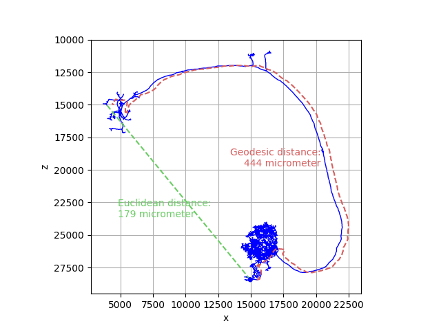
Euclidean distance is the straight-line distance between two points. Geodesic distance is measured along the arbor - following the neuron's cable. Because a neuron is rarely a straight line, the two differ, and questions like "how far is this terminal from the soma along the neuron?" call for the geodesic distance.
Euclidean distances are straightforward. Here we measure the average distance between a node and its parent (i.e. the sampling rate):
import numpy as np

# Get nodes but remove the root (has no parent)
nodes = nl[0].nodes[nl[0].nodes.parent_id > 0]

# Get the x/y/z coordinates of all nodes (except root)
node_locs = nodes[["x", "y", "z"]].values

# For each node, get its parent's location
parent_locs = (
    nl[0].nodes.set_index("node_id").loc[nodes.parent_id.values, ["x", "y", "z"]].values
)

# Calculate Euclidean distances
distances = np.sqrt(np.sum((node_locs - parent_locs) ** 2, axis=1))

# Use the neuron's units to convert into nm
distances = distances * nl[0].units

print(
    f"Mean distance between nodes: {np.mean(distances):.2f} (+/- {np.std(distances):.2f})"
)
Out:
Mean distance between nodes: 477.56 nanometer (+/- 361.10 nanometer)
For the distance between the soma and all terminal nodes we need the geodesic distance (see the box above) - the neuron is not a straight line. For single node-to-node queries, navis.dist_between is sufficient:
n = nl[0]

end = n.nodes[n.nodes.type == "end"].node_id.values[0]

d_geo = navis.dist_between(n, n.soma, end) * n.units

print(f"Euclidean distance between soma and terminal node {end}: {d_geo:.2f}")
Out:
Euclidean distance between soma and terminal node 465: 444096.16 nanometer
Visualizing the two distances:
import networkx as nx

# First we need to find the path between the soma and the terminal node
path = nx.shortest_path(n.graph.to_undirected(), n.soma, end)

# Get coordinates for the path
path_co = n.nodes.set_index("node_id").loc[path, ["x", "y", "z"]].copy()

# Add a small offset
path_co.x += 500
path_co.y -= 500

# Plot neuron
fig, ax = navis.plot2d(n, c="blue", method="2d", view=("x", "-z"))

# Add geodesic path
ax.plot(path_co.x, path_co.z, c="r", ls="--")

# Add Euclidean path
end_loc = n.nodes.set_index("node_id").loc[end, ["x", "y", "z"]]
soma_loc = n.nodes.set_index("node_id").loc[n.soma, ["x", "y", "z"]]
ax.plot([soma_loc.x, end_loc.x], [soma_loc.z, end_loc.z], c="g", ls="--")

d_eucl = np.sqrt(np.sum((end_loc - soma_loc) ** 2)) * n.units

# Annotate distances
_ = ax.text(
    x=0.1,
    y=0.3,
    s=f"Euclidean distance:\n{d_eucl.to_compact():.0f}",
    transform=ax.transAxes,
    c="g",
)
_ = ax.text(
    x=0.85,
    y=0.5,
    s=f"Geodesic distance:\n{d_geo.to_compact():.0f}",
    transform=ax.transAxes,
    c="r",
    ha="right",
)
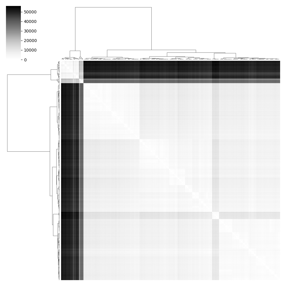
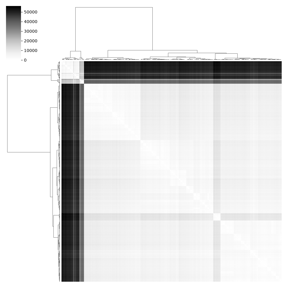
If you want to look at geodesic distances across many nodes, you should consider using navis.geodesic_matrix. To demonstrate, let's generate a geodesic distance matrix between all terminal nodes:
# Calculate distances from all end nodes to all other nodes
ends = n.nodes[n.nodes.type == "end"].node_id.values
m = navis.geodesic_matrix(n, from_=ends)

# Subset to only end-nodes-to-end_nodes
m = m.loc[ends, ends]

m.head()
Visualizing any clusters with a seaborn clustermap:
import seaborn as sns

from scipy.cluster.hierarchy import linkage
from scipy.spatial.distance import squareform

# Generate a linkage from the distances
Z = linkage(squareform(m, checks=False), method="ward")

# Plot
cm = sns.clustermap(m, cmap="Greys", col_linkage=Z, row_linkage=Z)

cm.ax_heatmap.set_xticks([])
cm.ax_heatmap.set_yticks([])
Out:
[]
As you can see in the heatmap, the dendrites and the axon nicely separate.
That's it for now! Please see the NBLAST tutorial for morphological comparisons using NBLAST and the API reference for a full list of morphology-related functions.
Total running time of the script: ( 0 minutes 3.797 seconds)
Download Python source code: tutorial_morpho_01_analyze.py