Note
Click here to download the full example code
Manipulate Morphology#
Prune, resample, smooth and reshape neuron morphology.
See the API reference for a complete list of available functions.
Some manipulations work on all (or most) neuron types; others only make sense for a specific type - rerooting, for example, only applies to a navis.TreeNeuron. As a rule of thumb, a generically named function like downsample_neuron accepts multiple types, while a specialized one like reroot_skeleton is type-specific. Depending on your data you may therefore need to convert between neuron types first.
This tutorial covers the operations below - the table doubles as an index and shows which neuron types each supports:
| Operation | TreeNeuron | MeshNeuron | Dotprops | VoxelNeuron |
|---|---|---|---|---|
Reroot (reroot_skeleton) | ✅ | — | — | — |
Downsample (downsample_neuron) | ✅ | ✅ | ✅ | ✅ |
Resample (resample_skeleton) | ✅ | — | — | — |
Smooth (smooth_skeleton / smooth_mesh / smooth_voxels) | ✅ | ✅ | — | ✅ |
Cut & prune (cut_skeleton, prune_twigs) | ✅ | ✅ | — | — |
Subset to volume (in_volume) | ✅ | ✅ | ✅ | ✅ |
Cutting or pruning a navis.MeshNeuron operates on its skeleton and propagates the changes back to the mesh, so the result may not be perfect (e.g. not watertight).
Rerooting#
navis.TreeNeurons are hierarchical trees and as such typically have a single "root" node (fragmented neurons will have multiple roots). The root is important because it is used as the reference/origin for a bunch of analyses such as Strahler order. Typically, you want the root to be the soma. Because the root is so important, TreeNeuron can be rerooted:
import navis

n = navis.example_neurons(1, kind="skeleton")
print(n.soma)
Out:
4177
.soma returns the node ID of the soma (if there is one) and can be used to reroot
navis.reroot_skeleton(n, n.soma, inplace=True)
Note
The root is implicitly also important for navis.MeshNeuron because we're using their skeleton representations for a couple operations/analyses!
Simplifying#
Downsampling/simplifying is handy before, say, plotting large lists of neurons. It works on all neuron types (see the table at the top), though the implementation differs per type.
For TreeNeurons downsampling means skipping N nodes (here 10):
sk = navis.example_neurons(n=1, kind="skeleton")
print(sk.n_nodes)
Out:
4465
sk_downsampled = navis.downsample_neuron(sk, downsampling_factor=10, inplace=False)
print(sk_downsampled.n_nodes)
Out:
1304
For MeshNeurons downsampling will reduce the number of faces by a factor of N:
me = navis.example_neurons(n=1, kind="mesh")
print(me.n_faces)
Out:
13054
me_downsampled = navis.downsample_neuron(me, downsampling_factor=10, inplace=False)
print(me_downsampled.n_faces)
Out:
1459
Note
Under the hood downsample_neuron calls navis.simplify_mesh for MeshNeurons. That function then requires one of the supported backends for mesh operations to be installed: Blender 3D, pymeshlab or open3d. If none is available, it will prompt you to install one.
Resampling#
TreeNeurons can also be "resampled" (up or down) to a given resolution (i.e. distance between nodes):
sk = navis.example_neurons(n=1, kind="skeleton")
print(sk.sampling_resolution * sk.units)
Out:
477.4501647949219 nanometer
Note that we can provide a unit ("1 micron") here because our neuron has units set:
sk_resampled = navis.resample_skeleton(sk, resample_to="1 micron", inplace=False)
print(sk_resampled.sampling_resolution * sk_resampled.units)
Out:
895.2661743164062 nanometer
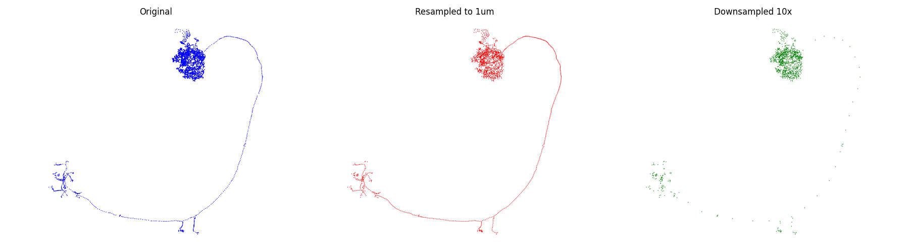
Comparing the original, resampled and downsampled skeletons side by side:
import matplotlib.pyplot as plt

nodes_original = sk.nodes[["x", "y", "z"]].values
nodes_downsampled = sk_downsampled.nodes[["x", "y", "z"]].values
nodes_resampled = sk_resampled.nodes[["x", "y", "z"]].values

fig, axes = plt.subplots(1, 3, figsize=(18, 5))

_ = navis.plot2d(
    nodes_original,
    method="2d",
    view=("x", "-z"),
    scatter_kws=dict(c="blue"),
    ax=axes[0],
)
_ = navis.plot2d(
    nodes_resampled,
    method="2d",
    view=("x", "-z"),
    scatter_kws=dict(c="red"),
    ax=axes[1],
)
_ = navis.plot2d(
    nodes_downsampled,
    method="2d",
    view=("x", "-z"),
    scatter_kws=dict(c="green"),
    ax=axes[2],
)

for ax, title in zip(axes, ["Original", "Resampled to 1um", "Downsampled 10x"]):
    ax.set_title(title, color="k")
    ax.invert_yaxis()
    ax.set_axis_off()

plt.tight_layout()
Tip
Click on the image to see it in full resolution.
As you can see the resampling increased the node density in the backbone and decreased it in the finer neurites to bring things on par. Downsampling just thinned out the nodes across the board.
Resampling regenerates node IDs
Nodes are not merely moved around to match the desired resolution - they are regenerated from scratch. As a consequence, the original node IDs are (with a few exceptions) all gone.
%%
Smoothing#
Smoothing works on all neuron types, but the approaches differ so much that each has its own function. Pick the tab for your neuron type:
navis.smooth_skeleton uses a rolling window along the linear segments:
sk = navis.example_neurons(n=1, kind="skeleton")
sk_smoothed = navis.smooth_skeleton(sk, window=5, inplace=False)
navis.smooth_mesh applies iterative rounds of Laplacian smoothing:
me = navis.example_neurons(n=1, kind="mesh")
me_smoothed = navis.smooth_mesh(me, iterations=5, inplace=False)
navis.smooth_voxels applies a Gaussian filter to the voxel grid:
vx = navis.voxelize(navis.example_neurons(n=1, kind="mesh"), pitch="1 micron")
vx_smoothed = navis.smooth_voxels(vx, sigma=2, inplace=False)
Running the skeleton smoother on a real neuron:
sk = navis.example_neurons(n=1, kind="skeleton")
sk_smoothed = navis.smooth_skeleton(sk, window=5, inplace=False)
sk_smoothed
Cutting & Pruning#
Cutting and pruning work best if there is a sense of topology which implicitly requires a skeleton. Many functions will also work on MeshNeurons though. That's because the operation is performed on their skeleton and changes are propagated back to the mesh. Fair warning though: this may not be perfect (e.g. the resulting mesh might not be watertight) - should be good enough for a first pass though!
Start with the simplest case: cutting a skeleton in two at a given node.
# Load the neuron
n = navis.example_neurons(1, kind="skeleton")

# Pick a node ID
cut_node_id = n.nodes.node_id.values[333]
distal, proximal = navis.cut_skeleton(n, cut_node_id)
Plot the two fragments:
# Note that we are using method='2d' here because that makes annotating the plot easier
fig, ax = distal.plot2d(color="cyan", method="2d", view=("x", "-z"))
fig, ax = proximal.plot2d(color="green", ax=ax, method="2d", view=("x", "-z"))

# Annotate cut point
cut_coords = distal.nodes.set_index("node_id").loc[distal.root, ["x", "z"]].values[0]
ax.annotate(
    "cut point",
    xy=(cut_coords[0], -cut_coords[1]),
    color="lightgrey",
    xytext=(cut_coords[0], -cut_coords[1] - 2000),
    va="center",
    ha="center",
    arrowprops=dict(shrink=0.1, width=2, color="lightgrey"),
)

plt.tight_layout()
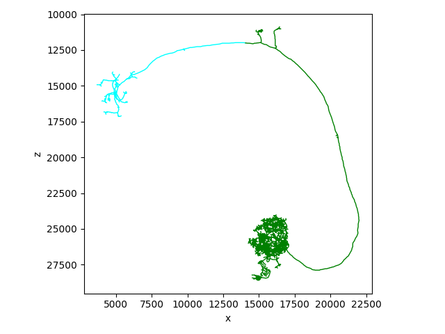
If instead of a node ID, you have an x/y/z coordinate where you want to cut: use the .snap method to find the closest node to that location:
node_id, dist = n.snap([14000, 16200, 12000])
print(f"Closest node: {node_id} at distance {dist * n.units:.2f} {n.units.units}")
Out:
Closest node: 334 at distance 565.69 nanometer nanometer
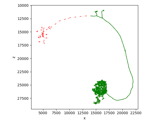
Instead of cutting a neuron in two, we can also just prune bits off:
n_pruned = n.prune_distal_to(cut_node_id, inplace=False)

cut_coords = n.nodes.set_index("node_id").loc[cut_node_id, ["x", "z"]].values

# Plot original neuron in red and with dotted line
fig, ax = n.plot2d(color="red", method="2d", linestyle=(0, (5, 10)), view=("x", "-z"))

# Plot remaining neurites in red
fig, ax = n_pruned.plot2d(color="green", method="2d", ax=ax, view=("x", "-z"), lw=1.2)

# Annotate cut point
ax.annotate(
    "cut point",
    xy=(cut_coords[0], -cut_coords[1]),
    color="lightgrey",
    xytext=(cut_coords[0], -cut_coords[1] - 2000),
    va="center",
    ha="center",
    arrowprops=dict(shrink=0.1, width=2, color="lightgrey"),
)

plt.tight_layout()
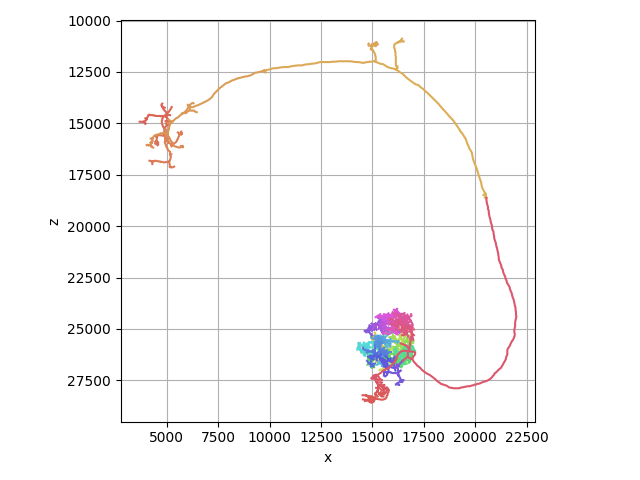
navis.cut_skeleton also takes multiple cut nodes, in case you want to chop your neuron into multiple pieces.
As an (extreme) example, let's cut a neuron at every single branch point:
n = navis.example_neurons(1, kind="skeleton")

branch_points = n.nodes[n.nodes.type == "branch"].node_id.values

cut = navis.cut_skeleton(n, branch_points)
cut.head()
# Plot neuron fragments
fig, ax = navis.plot2d(cut, linewidth=1.5, view=("x", "-z"))

plt.tight_layout()
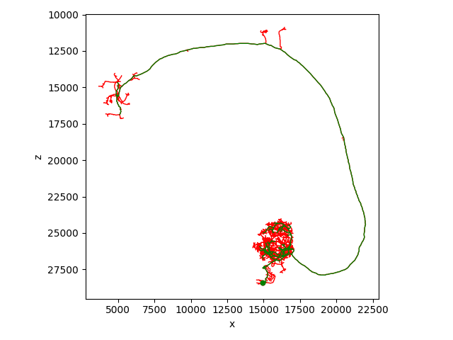
Next, pruning by Strahler index:
# Load a fresh skeleton
n = navis.example_neurons(1, kind="skeleton")

# Reroot to soma
n = n.reroot(n.soma)

# This will prune off terminal branches (the lowest two Strahler indices)
n_pruned = n.prune_by_strahler(to_prune=[1, 2], inplace=False)

# Plot original neurons in red
fig, ax = n.plot2d(color="red", view=('x', '-z'))

# Plot remaining neurites in green
fig, ax = n_pruned.plot2d(color="green", ax=ax, linewidth=1, view=("x", "-z"))

plt.tight_layout()
We can also turn this around and remove only the higher order branches. Let's use this example to show that we can also do this with MeshNeurons:
Load an example mesh neuron
m = navis.example_neurons(1, kind="mesh")

# This will prune to the just terminal branches
m_pruned = navis.prune_by_strahler(m, to_prune=range(3, 100), inplace=False)

# Plot original neuron in cyan
fig, ax = m.plot2d(color="cyan", figsize=(10, 10), view=("x", "-z"))

# Plot remaining neurites red
fig, ax = m_pruned.plot2d(color="red", ax=ax, view=("x", "-z"))

plt.tight_layout()

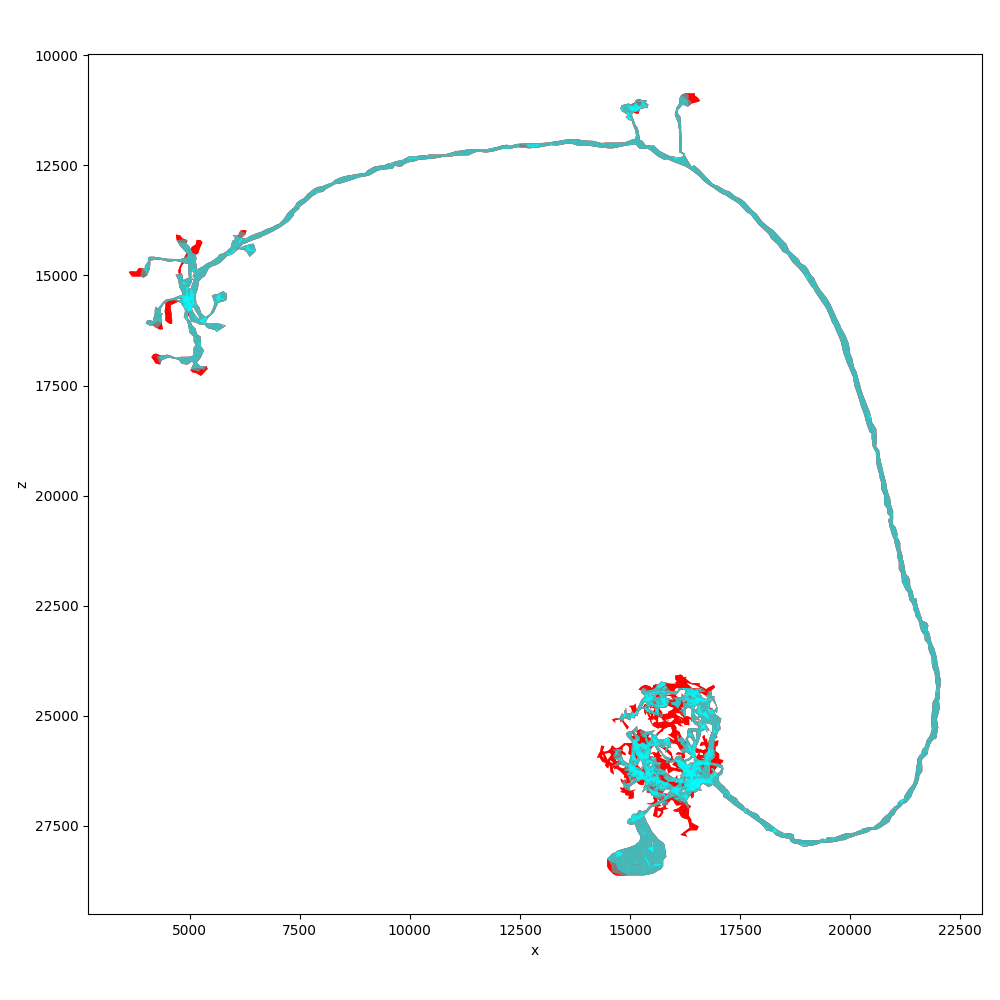
Alternatively, we can prune terminal branches based on size:
# This will prune all branches smaller than 10 microns
m_pruned = navis.prune_twigs(m, size="10 microns", inplace=False)

# Plot original neuron in red
fig, ax = m.plot2d(color="red", figsize=(10, 10), view=("x", "-z"))

# Plot remaining neurites in cyan
fig, ax = m_pruned.plot2d(
    color="cyan", ax=ax, linewidth=0.75, alpha=0.5, view=("x", "-z")
)

plt.tight_layout()
Intersecting with Volumes#
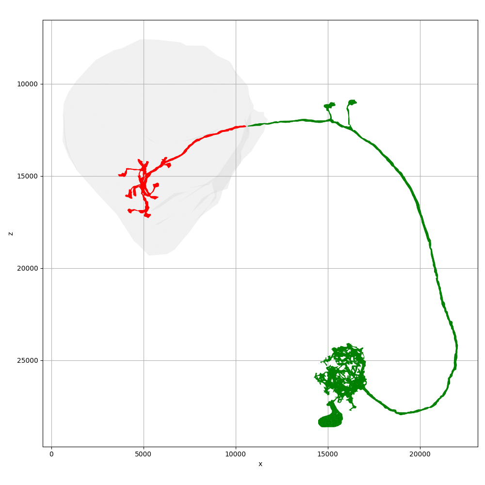
We can also intersect neurons with navis.Volume (and trimesh.Trimesh for that matter). This is useful e.g. to subset a neuron to a certain brain region:
Load an example navis.Volume
lh = navis.example_volume("LH")

# Prune by volume
m_lh = navis.in_volume(m, lh, inplace=False)
m_outside_lh = navis.in_volume(m, lh, mode="OUT", inplace=False)
And plot!
Plot pruned branches neuron in green
fig, ax = navis.plot2d(
    [m_lh, m_outside_lh, lh], color=["red", "green"], figsize=(10, 10), view=("x", "-z")
)

plt.tight_layout()
As the table at the top of this tutorial shows, not every operation applies to every neuron type: Dotprops and VoxelNeurons can't be cut, for example, but they can be subset to a volume. See the API reference for the full matrix.
# Note that [`navis.in_volume`][] also works with arbitrary spatial data (i.e. `(N, 3)` arrays of x/y/z locations):
Get the connectors for one of our above skeletons
cn = sk.connectors

# Add a column that tells us which connectors are in the LH volume
cn["in_lh"] = navis.in_volume(cn[["x", "y", "z"]].values, lh)
cn.head()
Count the number of connectors (pre and post) in- and outside the LH:
cn.groupby(["type", "in_lh"]).size()
Out:
type  in_lh
post  False    1978
      True      106
pre   False     325
      True      296
dtype: int64
About half the presynapses are in the LH (most of the rest will be in the MB calyx). The large majority of postsynapses are outside the LH in the antennal lobe where this neuron has its dendrites.
That's it for now! Please see the NBLAST tutorial for morphological comparisons using NBLAST and the API reference for a full list of morphology-related functions.
Total running time of the script: ( 0 minutes 11.758 seconds)
Download Python source code: tutorial_morpho_00_manipulate.py
Download Jupyter notebook: tutorial_morpho_00_manipulate.ipynb