Note
Click here to download the full example code
neuPrint#
Query and fetch neurons and connectivity from a neuPrint server.
NeuPrint is a service for presenting and analyzing connectomics data. It is used to host, for example, the Janelia EM reconstructions from a Drosophila hemibrain at https://neuprint.janelia.org/.
neuprint-python is a Python library that lets you query data directly from a neuPrint server. You can install it from PyPI:
pip3 install neuprint-python
navis.interfaces.neuprint wraps neuprint-python and adds a few new functions to fetch and convert data into NAVis objects.
Requires network access and a token
This tutorial talks to a live neuPrint server, so it needs an internet connection. You will also need a neuPrint account and an API token - see the "Authentication" note below for how to set it.
Import navis
import navis

# Import neuprint wrapper by navis
import navis.interfaces.neuprint as neu
Set up the connection#
Authentication
Pass your API token directly via token=..., or store it as a NEUPRINT_APPLICATION_CREDENTIALS environment variable. The latter is the recommended approach and the one we use here.
client = neu.Client(
    "https://neuprint.janelia.org/",
    # token="MYLONGTOKEN"  # use this to instead pass your token directly
    dataset="hemibrain:v1.2.1",
)
You can use all of neuprint's functions:
mbons, roi_info = neu.fetch_neurons(
    neu.SegmentCriteria(instance=".*MBON.*", regex=True)
)
mbons.head(3)
On top of neuprint-python's own functions, NAVis adds three that return NAVis objects:
| Function | Returns |
|---|---|
fetch_roi | a navis.Volume from a ROI |
fetch_skeletons | fully-fledged navis.TreeNeurons - nodes, synapses, soma and all |
fetch_mesh_neuron | navis.MeshNeurons - including synapses |
Start by fetching the mesh for the right mushroom body ROI:
mb = neu.fetch_roi("MB(R)")
mb
Out:
<navis.Volume(name=MB(R), units=1 dimensionless, color=(0.85, 0.85, 0.85, 0.2), vertices.shape=(57913, 3), faces.shape=(115856, 3))>
Next, let's fetch the skeletons of all right MBONs:
mbon_skeletons = neu.fetch_skeletons(
    neu.SegmentCriteria(instance=".*MBON.*_R", regex=True), with_synapses=True
)
mbon_skeletons.head()
Out:
  0%|          | 0/1 [00:00<?, ?it/s]


  0%|          | 0/1 [00:00<?, ?it/s]


  0%|          | 0/1 [00:00<?, ?it/s]


  0%|          | 0/1 [00:00<?, ?it/s]


  0%|          | 0/1 [00:00<?, ?it/s]

100%|##########| 1/1 [00:00<00:00,  7.64it/s]
100%|##########| 1/1 [00:00<00:00,  7.64it/s]


  0%|          | 0/1 [00:00<?, ?it/s]


100%|##########| 1/1 [00:00<00:00,  5.46it/s]
100%|##########| 1/1 [00:00<00:00,  5.46it/s]

100%|##########| 1/1 [00:00<00:00, 11.40it/s]


  0%|          | 0/1 [00:00<?, ?it/s]


  0%|          | 0/1 [00:00<?, ?it/s]


100%|##########| 1/1 [00:00<00:00,  2.41it/s]
100%|##########| 1/1 [00:00<00:00,  2.41it/s]


100%|##########| 1/1 [00:00<00:00,  4.80it/s]
100%|##########| 1/1 [00:00<00:00,  4.80it/s]


100%|##########| 1/1 [00:00<00:00,  1.63it/s]
100%|##########| 1/1 [00:00<00:00,  1.63it/s]


100%|##########| 1/1 [00:00<00:00,  2.33it/s]
100%|##########| 1/1 [00:00<00:00,  2.33it/s]


  0%|          | 0/1 [00:00<?, ?it/s]


100%|##########| 1/1 [00:00<00:00,  1.01it/s]
100%|##########| 1/1 [00:00<00:00,  1.01it/s]


100%|##########| 1/1 [00:00<00:00,  5.65it/s]
100%|##########| 1/1 [00:00<00:00,  5.65it/s]


  0%|          | 0/1 [00:00<?, ?it/s]


  0%|          | 0/1 [00:00<?, ?it/s]


  0%|          | 0/1 [00:00<?, ?it/s]


  0%|          | 0/1 [00:00<?, ?it/s]


  0%|          | 0/1 [00:00<?, ?it/s]


100%|##########| 1/1 [00:00<00:00,  9.58it/s]
100%|##########| 1/1 [00:00<00:00,  9.57it/s]


100%|##########| 1/1 [00:00<00:00,  4.38it/s]
100%|##########| 1/1 [00:00<00:00,  4.38it/s]


  0%|          | 0/1 [00:00<?, ?it/s]


  0%|          | 0/1 [00:00<?, ?it/s]
100%|##########| 1/1 [00:00<00:00, 22.50it/s]


100%|##########| 1/1 [00:00<00:00,  1.79it/s]
100%|##########| 1/1 [00:00<00:00,  1.79it/s]


  0%|          | 0/1 [00:00<?, ?it/s]


100%|##########| 1/1 [00:00<00:00,  1.44it/s]
100%|##########| 1/1 [00:00<00:00,  1.44it/s]


100%|##########| 1/1 [00:00<00:00,  4.62it/s]
100%|##########| 1/1 [00:00<00:00,  4.62it/s]


100%|##########| 1/1 [00:00<00:00,  1.20it/s]
100%|##########| 1/1 [00:00<00:00,  1.20it/s]


  0%|          | 0/1 [00:00<?, ?it/s]


  0%|          | 0/1 [00:00<?, ?it/s]


  0%|          | 0/1 [00:00<?, ?it/s]


  0%|          | 0/1 [00:00<?, ?it/s]
100%|##########| 1/1 [00:00<00:00, 12.48it/s]

100%|##########| 1/1 [00:00<00:00, 13.01it/s]


  0%|          | 0/1 [00:00<?, ?it/s]


100%|##########| 1/1 [00:01<00:00,  1.02s/it]
100%|##########| 1/1 [00:01<00:00,  1.02s/it]


100%|##########| 1/1 [00:00<00:00,  2.39it/s]
100%|##########| 1/1 [00:00<00:00,  2.39it/s]


100%|##########| 1/1 [00:00<00:00,  8.44it/s]
100%|##########| 1/1 [00:00<00:00,  8.43it/s]


  0%|          | 0/1 [00:00<?, ?it/s]


100%|##########| 1/1 [00:00<00:00,  1.66it/s]
100%|##########| 1/1 [00:00<00:00,  1.66it/s]


  0%|          | 0/1 [00:00<?, ?it/s]


  0%|          | 0/1 [00:00<?, ?it/s]


  0%|          | 0/1 [00:00<?, ?it/s]


  0%|          | 0/1 [00:00<?, ?it/s]
100%|##########| 1/1 [00:00<00:00, 12.14it/s]


100%|##########| 1/1 [00:00<00:00,  2.89it/s]
100%|##########| 1/1 [00:00<00:00,  2.89it/s]


  0%|          | 0/1 [00:00<?, ?it/s]


100%|##########| 1/1 [00:00<00:00,  3.29it/s]
100%|##########| 1/1 [00:00<00:00,  3.29it/s]


100%|##########| 1/1 [00:00<00:00,  2.71it/s]
100%|##########| 1/1 [00:00<00:00,  2.71it/s]


  0%|          | 0/1 [00:00<?, ?it/s]


100%|##########| 1/1 [00:00<00:00,  1.85it/s]
100%|##########| 1/1 [00:00<00:00,  1.85it/s]


100%|##########| 1/1 [00:00<00:00,  2.17it/s]
100%|##########| 1/1 [00:00<00:00,  2.17it/s]


  0%|          | 0/1 [00:00<?, ?it/s]


  0%|          | 0/1 [00:00<?, ?it/s]


  0%|          | 0/1 [00:00<?, ?it/s]


100%|##########| 1/1 [00:00<00:00,  2.19it/s]
100%|##########| 1/1 [00:00<00:00,  2.19it/s]


  0%|          | 0/1 [00:00<?, ?it/s]


  0%|          | 0/1 [00:00<?, ?it/s]


100%|##########| 1/1 [00:00<00:00,  2.70it/s]
100%|##########| 1/1 [00:00<00:00,  2.70it/s]


100%|##########| 1/1 [00:00<00:00,  5.19it/s]
100%|##########| 1/1 [00:00<00:00,  5.18it/s]


  0%|          | 0/1 [00:00<?, ?it/s]


  0%|          | 0/1 [00:00<?, ?it/s]


100%|##########| 1/1 [00:00<00:00,  1.91it/s]
100%|##########| 1/1 [00:00<00:00,  1.91it/s]


100%|##########| 1/1 [00:00<00:00,  6.13it/s]
100%|##########| 1/1 [00:00<00:00,  6.13it/s]


100%|##########| 1/1 [00:01<00:00,  1.25s/it]
100%|##########| 1/1 [00:01<00:00,  1.25s/it]


100%|##########| 1/1 [00:01<00:00,  1.68s/it]
100%|##########| 1/1 [00:01<00:00,  1.68s/it]


  0%|          | 0/1 [00:00<?, ?it/s]


100%|##########| 1/1 [00:01<00:00,  1.26s/it]
100%|##########| 1/1 [00:01<00:00,  1.26s/it]

100%|##########| 1/1 [00:00<00:00, 10.95it/s]


  0%|          | 0/1 [00:00<?, ?it/s]


  0%|          | 0/1 [00:00<?, ?it/s]


  0%|          | 0/1 [00:00<?, ?it/s]


  0%|          | 0/1 [00:00<?, ?it/s]


  0%|          | 0/1 [00:00<?, ?it/s]


100%|##########| 1/1 [00:00<00:00,  3.04it/s]
100%|##########| 1/1 [00:00<00:00,  3.04it/s]


100%|##########| 1/1 [00:00<00:00,  1.92it/s]
100%|##########| 1/1 [00:00<00:00,  1.92it/s]


100%|##########| 1/1 [00:00<00:00,  1.89it/s]
100%|##########| 1/1 [00:00<00:00,  1.89it/s]


100%|##########| 1/1 [00:00<00:00,  1.42it/s]
100%|##########| 1/1 [00:00<00:00,  1.42it/s]


  0%|          | 0/1 [00:00<?, ?it/s]


100%|##########| 1/1 [00:00<00:00,  1.19it/s]
100%|##########| 1/1 [00:00<00:00,  1.19it/s]


  0%|          | 0/1 [00:00<?, ?it/s]


100%|##########| 1/1 [00:00<00:00,  3.44it/s]
100%|##########| 1/1 [00:00<00:00,  3.44it/s]


100%|##########| 1/1 [00:00<00:00,  1.91it/s]
100%|##########| 1/1 [00:00<00:00,  1.91it/s]
Co-visualize the MBONs and the MB volume:
navis.plot3d(
    [mbon_skeletons[0], mb],
    legend=False,  # Hide the legend (more space for the plot)
)
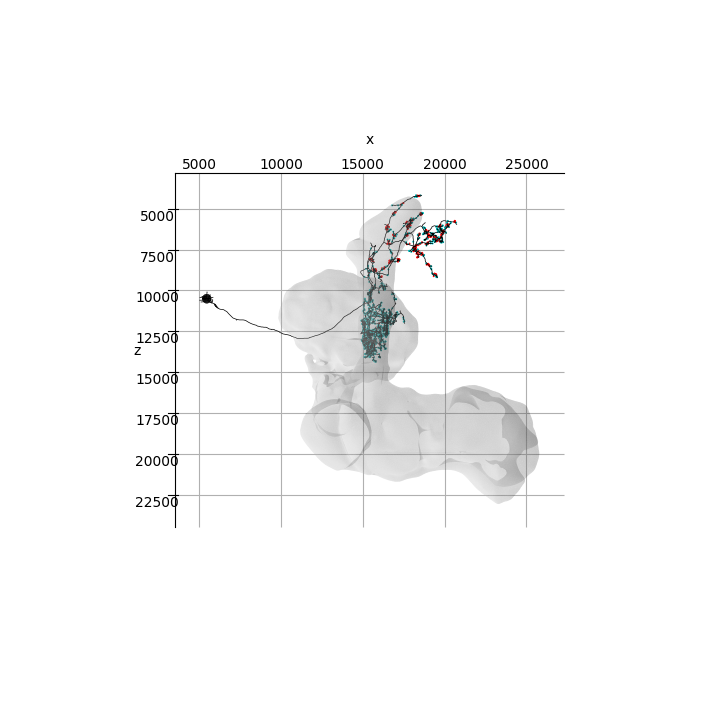
Last (but not least), let's make a 2d plot for the tutorial's thumbnail:
import matplotlib.pyplot as plt

fig, ax = navis.plot2d(
    [mbon_skeletons[0], mb],
    c=(0, 0, 0, 1),  # Make the neuron black
    method="3d",
    connectors=True,
    linewidth=0.5,  # Make neuron a bit thinner to emphasize the synapses
    view=("x", "-z"),
)

plt.tight_layout()
All NAVis functions for analysis & visualization should work on these neurons. If not, please open an issue on Github.
Total running time of the script: ( 0 minutes 12.231 seconds)
Download Python source code: tutorial_remote_00_neuprint.py
Download Jupyter notebook: tutorial_remote_00_neuprint.ipynb