Note
Click here to download the full example code
NEURON simulator#
Run compartment-model simulations of neurons and networks via the NEURON simulator.
NEURON is a simulation environment for modeling neurons and networks. It's powerful but fairly low-level, so building models tends to involve a lot of boilerplate. Higher-level wrappers like NetPyNE exist, but they're geared towards probabilistic models (e.g. "create 100 neurons with a 10% chance of connecting") rather than the well-defined morphology and connectivity you get from connectomics.
NAVis doesn't try to be a full simulation suite. Instead it fills a gap for people working with non-probabilistic data (e.g. from connectomics), giving you an entry point to get started with simple models and build from there. There are two types of models:
-
CompartmentModel
Model an individual neuron (you can also connect several) from a skeleton.
-
PointNetwork
Model a network of point-process neurons from an edge list.
Compartment models#
A CompartmentModel represents a single neuron (although you can connect multiple of these neurons) and is constructed from a skeleton (i.e. navis.TreeNeuron, see also navis.conversion.mesh2skeleton). The full pipeline looks like this:
graph LR
    A[Load skeleton] --> B[Build model]
    B --> C[Label axon & dendrite]
    C --> D[Insert mechanisms]
    D --> E[Add recordings]
    E --> F[Add stimulation]
    F --> G[Run simulation]
    G --> H[Plot results]
import navis
import neuron
import navis.interfaces.neuron as nrn
# Load one of the example neurons (a Drosophila projection neuron from the hemibrain connectome)
# Note the conversion to microns!
n = navis.example_neurons(1).convert_units("um")
# Here we manually corrected the soma
n.soma = 20
# Reroot to the soma
n.reroot(n.soma, inplace=True)
# Create the compartment model
cmp = nrn.CompartmentModel(n, res=10)
NEURON compartment models are collections of connected linear segments, and each segment can carry its own properties and mechanisms. Here we set three biophysical constants for the whole neuron, using values from Tobin et al. (2017):
cmp.Ra = 266.1                         # (1)!
cmp.cm = 0.8                           # (2)!
cmp.insert("pas", g=1 / 20800, e=-60)  # (3)!
- Specific axial resistivity, in
Ohm cm. - Specific membrane capacitance, in
mF / cm**2. - Passive ("leak") membrane properties:
gis the specific leak conductance (1/Rm, whereRmis the specific membrane resistance inOhm cm**2) andeis the leak reversal potential.
# Set axial resistivity, membrane capacitance and passive membrane properties
cmp.Ra = 266.1
cmp.cm = 0.8
cmp.insert("pas", g=1 / 20800, e=-60)
At this point we already have a passive model of our Drosophila projection neuron. Next, we will determine what's axon and what's dendrite, and add a Hodgkin & Huxley mechanism so we have some actual action potentials to observe.
This will also illustrate one of the features of CompartmentModels: we keep a correspondence to the original skeleton via node (and connector) IDs. This allows you to modify, stimulate at or record from parts of the compartment model by using node IDs.
# Label axon/dendrite
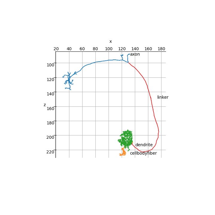
navis.split_axon_dendrite(n, label_only=True, cellbodyfiber="soma")

n.nodes.head()
A quick visualization
import matplotlib.pyplot as plt

fig, ax = navis.plot2d(
    n, color_by="compartment", palette="tab10", lw=1.5, method="3d", view=("x", "-z")
)

# Label compartments
for l in n.nodes.compartment.unique():
    loc = n.nodes.loc[n.nodes.compartment == l, ["x", "y", "z"]].values[-1]
    ax.text(loc[0] + 10, loc[1], loc[2], l)

plt.tight_layout()
Note
A little excursion about how NEURON represents neurons before we add the Hodgkin & Huxley (HH) mechanism: neurons consist of linear "sections" while individual (continuous) positions along each section are called "segments". That distinction is important because our skeleton nodes correspond to segments but a mechanism such as HH is applied for entire sections.
# Collect axon nodes
axon_nodes = n.nodes.loc[n.nodes.compartment.isin(["axon", "linker"]), "node_id"].values

# Get the sections for the given nodes
axon_secs = list(set(cmp.get_node_section(axon_nodes)))

# Insert HH mechanism at the given sections
cmp.insert("hh", subset=axon_secs)
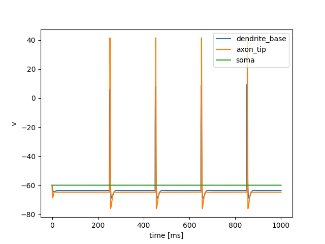
Next we actually have to do something with our compartment model. For that we will add three voltage recorders: one at the soma, one at the base of the dendrites and one at the tip of the axon.
Recordings and stimulations work via segments (as opposed to sections for mechanisms) -> hence we can use node IDs directly here
Let's determine the tip of the axon and base of the dendrites programmatically using the geodesic distance:
dists = navis.geodesic_matrix(n, from_=n.soma)

# Sort by distance from soma
dists = dists.iloc[0].sort_values()

dists.head(10)
Out:
20      0.000000
21      0.455753
19      0.633259
2409    0.836538
22      1.095767
18      1.113258
23      1.415775
2410    1.474030
24      1.692905
17      2.032377
Name: 20, dtype: float32
# Find the closest "dendrite" and the most distal "axon" node
dend = n.nodes[n.nodes.compartment == "dendrite"].node_id.values
dend_base = dists.index[dists.index.isin(dend)][0]
print(f"Node at the base of the dendrites: {dend_base}")

axo = n.nodes[n.nodes.compartment == "axon"].node_id.values
axo_tip = dists.index[dists.index.isin(axo)][-1]
print(f"Node at the tip of the axon: {axo_tip}")
Out:
Node at the base of the dendrites: 467
Node at the tip of the axon: 4384
# Add voltage recordings
cmp.add_voltage_record(dend_base, label="dendrite_base")
cmp.add_voltage_record(axo_tip, label="axon_tip")
cmp.add_voltage_record(n.soma, label="soma")
Last but not least we need to provide some input to our neuron otherwise it will just sit there doing nothing. We can add a current injection, trigger some synaptic currents or add a leak current. Let's simulate some synaptic inputs:
# Get dendritic postsynapses
post = n.postsynapses[n.postsynapses.compartment == "dendrite"]
post.head()
# Here we will open successively more synapses over 5 stimulations
for i in range(5):
    # Onset for this stimulation
    start = 50 + i * 200
    # Number of synapses to activate
    n_syn = i * 5
    cmp.add_synaptic_current(
        where=post.node_id.unique()[0:n_syn], start=start, max_syn_cond=0.1, rev_pot=-10
    )
# Now we can run our simulation for 1000ms
# (this is equivalent to neuron.h.finitialize + neuron.h.continuerun)
cmp.run_simulation(1000, v_init=-60)
The compartment model has a quick & dirty way of plotting the results:
# Plot the results
axes = cmp.plot_results()
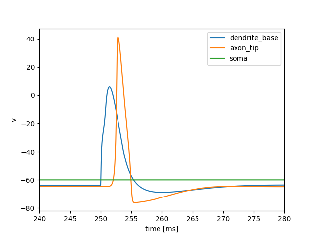
# Plot again and zoom in on one spike
axes = cmp.plot_results()
axes[0].set_xlim(240, 280)
Out:
(240.0, 280.0)
As you can see we get a nice depolarization at the base of the dendrites which elicits an action potential that we can measure in the tips of the axon. Because in our model the cell body fiber (i.e. the neurite that connects the soma to the base of the dendrites) is passive, the depolarization of a single spike attenuates before it reaches the soma.
Alternatively, you can access the recorded values directly like so:
cmp.records
Out:
{'v': {'dendrite_base': Vector[0], 'axon_tip': Vector[1], 'soma': Vector[2]}}
cmp.records["v"]["dendrite_base"].as_numpy()
Out:
array([-60.        , -60.05746836, -60.10429959, ..., -63.74603203,
       -63.74603203, -63.74603203], shape=(40001,))
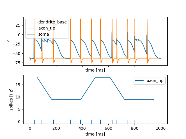
Next, let's try to simulate some noisy input where the presynaptic neuron spikes multiple times:
# First we need to reset our model (by re-assigning `cmp` the old model will be garbage-collected)
cmp = nrn.CompartmentModel(n, res=10)

# Set properties and mechanisms
cmp.Ra, cmp.cm = 266.1, 0.8
cmp.insert("pas", g=1 / 20800, e=-60)
axon_secs = list(set(cmp.get_node_section(axon_nodes)))
cmp.insert("hh", subset=axon_secs)

# Add recording
cmp.add_voltage_record(dend_base, label="dendrite_base")
cmp.add_voltage_record(axo_tip, label="axon_tip")
cmp.add_voltage_record(n.soma, label="soma")

# Also add a spike counter at the axon
cmp.add_spike_detector(axo_tip, label="axon_tip")

# Now add a noisy preinput to say 20 dendritic postsynapses
post = n.connectors[
    (n.connectors.compartment == "dendrite") & (n.connectors.type == "post")
]
cmp.add_synaptic_input(
    post.node_id.unique()[0:20],
    spike_no=20,  # produce 20 presynaptic spikes
    spike_int=50,  # with an average interval of 50ms: 20 * 50ms = over 1s
    spike_noise=1,  # very noisy!
    cn_weight=0.04,
)
# Run for 1s
cmp.run_simulation(1000, v_init=-60)
# Plot results
axes = cmp.plot_results()
axes[1].set_ylabel("spikes [Hz]")
Out:
Text(93.44444444444443, 0.5, 'spikes [Hz]')
Note how we still don't see a depolarization in the soma? While that might be a genuine biological feature of this neuron, I suspect there is something wrong with the radii along the cell body fiber - perhaps a pinch point somewhere? This just illustrates that good skeletons are paramount and you should critically inspect the results of your models.
Many methods in CompartmentModel use sensible defaults so you get some sort of effect out of the box. As you fit a model to real-world data, you'll want to tune the parameters.
Discover the parameters
Every method documents its options - check the help for any of them, e.g.:
help(cmp.add_synaptic_input)
Point Networks#
While you can link together multiple compartment models to simulate networks this quickly becomes prohibitively slow to run. For larger networks it can be sufficient to model each neuron as a single "point process". PointNetwork lets you quickly create such a network from an edge list.
In this tutorial we will use toy data but it is just as straightforward to plug in real data:
# First create a small 3 way network where one of the neurons (B) is inhibitory
import pandas as pd

edges = pd.DataFrame([])
edges["source"] = ["A", "B"]
edges["target"] = ["C", "C"]
edges["weight"] = [0.5, -1]
edges
# Next initialize network from edge list
net = nrn.PointNetwork.from_edge_list(edges, model="IntFire4")
net
Out:
PointNetwork<neurons=3,edges=2>
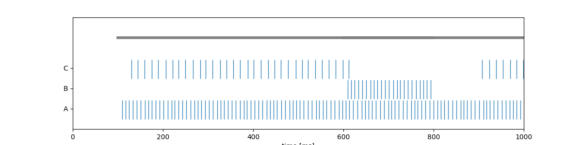
So far, our network won't do anything because it doesn't have any input. Let's add an input to neurons A and B, and try that out:
# Add the stimulus
net.add_stimulus("A", start=100, stop=1000, frequency=100, randomness=0)
net.add_stimulus("B", start=600, stop=800, frequency=100, randomness=0)

# Run simulation
net.run_simulation(1000)
# Plot
ax = net.plot_raster(backend="matplotlib", label=True)

ax.set_xlim(0, 1000)
Out:
(0.0, 1000.0)
This toy example worked quite well: spikes in neuron A elicit occasional spikes in C via temporal summation. Activity in the inhibitory neuron B hyperpolarizes C and it stops firing until well after activity in B has ceased.
The NEURON interface is a very recent addition and it might well change in the future (or become its own package). Functionality is also still limited and while I don't intend to write a feature-complete wrapper for NEURON, I do welcome feature requests or contributions on Github.
Links#
- Model DB contains various published
NEURONmodels and mechanisms - NetPyNE wraps
NEURONand provides high-level syntax to create models
Total running time of the script: ( 0 minutes 7.525 seconds)
Download Python source code: tutorial_interfaces_00_neuron.py
Download Jupyter notebook: tutorial_interfaces_00_neuron.ipynb