Note
Click here to download the full example code
Neuroglancer & CloudVolume#
Pull neurons and meshes from Neuroglancer sources via CloudVolume.
Neuroglancer is a WebGL-based viewer for volumetric data. You may have used it to browse some of the recent large EM datasets. If you want to programmatically access/download these data, you need CloudVolume. CloudVolume is an excellent Python library developed by William Silversmith (Seung lab, Princeton) and others. While CloudVolume is not directly related to Neuroglancer, it shares much of its functionality. As a rule of thumb: if you can view a dataset in Neuroglancer, you can download that data using CloudVolume. For example:
| Dataset | Description |
|---|---|
| FlyWire | Segmentation of an entire Drosophila brain. Very much work in progress; you'll need to register and apply for access. See FAFBseg for a mature NAVis-based interface. |
| Google FFN | Google's flood-filling segmentation of an entire Drosophila brain. |
| MICrONS | The Allen Institute's datasets - see the dedicated MICrONS tutorial. |
| hemibrain | The Janelia hemibrain connectome. |
You can find the source for the data you want to access by right-clicking on the layer in question and selecting the "Source" tab on the right:
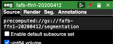
CloudVolume supports pretty much all the backends/data formats that neuroglancer does. You can use it to programmatically query the segmentation itself, and to fetch meshes and skeletons (if available). NAVis & friends provide simple interfaces for some of the datasets (see e.g. the neuPrint and the MICrONs tutorials) but there is also some lower-level option to pull neurons into NAVis via CloudVolume.
First of all, you will want to make sure cloud-volume is installed and up-to-date:
pip install cloud-volume -U
Network access
This tutorial downloads data from remote Neuroglancer sources, so it needs an internet connection. Some datasets (e.g. FlyWire) additionally require you to register and authenticate.
Once that's done we can start pulling data using cloud-volume. In this example here, we will use the Google segmentation of the FAFB dataset:
import navis
import cloudvolume as cv

# This tutorial pulls from a remote source that may be unreachable when the docs
# are built, so we pin a static thumbnail rather than rely on a scraped figure.
Patch before you connect
navis.patch_cloudvolume monkey-patches cloudvolume so that its get() methods return NAVis neurons. Run it before you create the CloudVolume object, and only once per session.
# This needs to be run only once at the beginning of each session
navis.patch_cloudvolume()
Now we can connect to our data source. Here we connect to the Google segmentation of the FAFB dataset:
# Don't forget to set `use_https=True` to avoid having to setup Google credentials!
vol = cv.CloudVolume(
    "precomputed://gs://fafb-ffn1-20200412/segmentation", use_https=True, progress=False
)
Fetch neuron meshes:
# Setting `as_navis=True` will get us MeshNeurons
m = vol.mesh.get([4335355146, 2913913713, 2137190164, 2268989790], as_navis=True, lod=3)
m
Shortcut
Instead of vol.mesh.get(..., as_navis=True) you can also use the shortcut vol.mesh.get_navis(...) which is equivalent.
Plot!
navis.plot3d(
    m,
    legend_orientation="h",  # few neurons, so we can afford a horizontal legend
)
# And one 2D plot (for the tutorial thumbnail)
import matplotlib.pyplot as plt

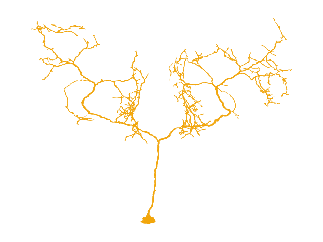
fig, ax = navis.plot2d(m[1], method="2d", view=("x", "-y"))
ax.set_axis_off()
ax.grid(False)
plt.tight_layout()
This also works for skeletons:
sk = vol.skeleton.get([4335355146, 2913913713, 2137190164, 2268989790], as_navis=True)
sk
Note that not all datasets contain precomputed skeletons! In that case you could download the meshes and use navis.skeletonize to skeletonize them.
Try it out!
If you are working a lot with NeuroGlancer and need to e.g. generate or parse URLs, you might want to check out the nglscenes package.
Total running time of the script: ( 0 minutes 4.689 seconds)
Download Python source code: tutorial_remote_01_cloudvolume.py
Download Jupyter notebook: tutorial_remote_01_cloudvolume.ipynb