Note
Click here to download the full example code
Visualize NEURON model#
Visualize a NEURON compartment model in 3D.
We will jump right in, so please make sure to have a look at the introductory NEURON tutorial first.
Setup the model#
Same setup as the previous tutorial
The cell below repeats the compartment-model setup from the introductory NEURON tutorial: load an example neuron, set the biophysical constants, label axon and dendrite, and insert the passive and Hodgkin-Huxley mechanisms. It has to run so the later cells work, but you can skip reading it if you've been through that tutorial.
import navis
import neuron
import navis.interfaces.neuron as nrn
# Load one of the example neurons (a Drosophila projection neuron from the hemibrain connectome)
# Note the conversion to microns!
n = navis.example_neurons(1).convert_units("um")
# Here we manually corrected the soma
n.soma = 20
# Reroot to the soma
n.reroot(n.soma, inplace=True)
# Create the compartment model
cmp = nrn.CompartmentModel(n, res=10)
# Set the specific axial resistivity for the entire neuron in Ohm cm
cmp.Ra = 266.1
# Set the specific membrane capacitance in mF / cm**2
cmp.cm = 0.8
# Add passive membrane properties for the entire neuron
cmp.insert(
"pas",
g=1
/ 20800, # specific leakage conductance = 1/Rm; Rm = specific membrane resistance in Ohm cm**2
e=-60, # leakage reverse potential
)
# Label axon/dendrite
navis.split_axon_dendrite(n, label_only=True, cellbodyfiber="soma")
# Collect axon nodes
axon_nodes = n.nodes.loc[n.nodes.compartment.isin(["axon", "linker"]), "node_id"].values
# Get the sections for the given nodes
axon_secs = list(set(cmp.get_node_section(axon_nodes)))
# Insert HH mechanism at the given sections
cmp.insert("hh", subset=axon_secs)
Next, we will add a voltage recording at every single node of the neuron.
cmp.add_voltage_record(n.nodes.node_id.values)
Last but not least, we will add a synaptic input at some dendritic postsynapses of the neuron.
# Get dendritic postsynapses
post = n.postsynapses[n.postsynapses.compartment == "dendrite"]
# Add synaptic input to the first 10 postsynapses after 2 ms
cmp.add_synaptic_current(where=post.node_id.unique()[0:10], start=2, max_syn_cond=0.1, rev_pot=-10)
Now we can run our simulation for 100ms
# This is equivalent to neuron.h.finitialize + neuron.h.continuerun
cmp.run_simulation(100, v_init=-60)
Collect the data#
To visualize and animate, we will collect the results into a pandas DataFrame
import numpy as np
import pandas as pd
# Collect the voltage recordings at each node
records = pd.DataFrame(np.vstack([r.as_numpy() for r in cmp.records['v'].values()]), index=list(cmp.records['v'].keys()))
# Reindex to make sure it matches the node table
records = records.reindex(n.nodes.node_id)
records.head()
Visualize#
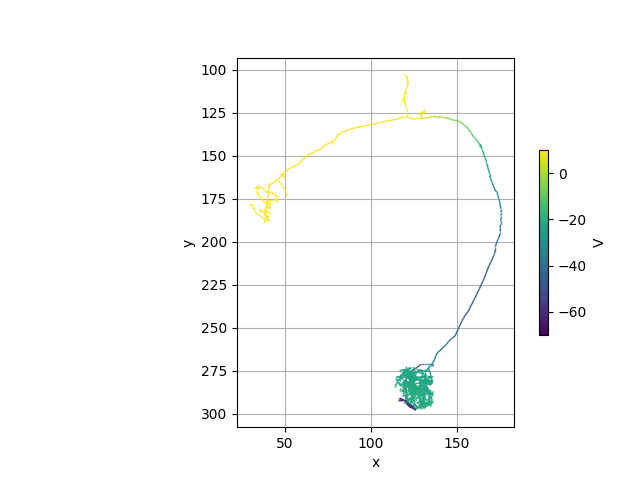
Let's first visualize a single snapshot of the neuron at time t=5ms:
# The interval for each step is 0.025ms by default
print(neuron.h.dt)
Out:
0.025
Add a new column to the node table for time t=5ms
n.nodes['v'] = records.loc[:, int(5 / 0.025)].values
# Plot
fig, ax = navis.plot2d(
n,
method="2d",
color_by="v", # color by the voltage column
palette="viridis",
vmin = -70,
vmax = 10,
view=('x', '-y')
)
# Manually add a colorbar
import matplotlib.pyplot as plt
from matplotlib.cm import ScalarMappable
sm = ScalarMappable(norm=plt.Normalize(vmin=-70, vmax=10), cmap='viridis')
_ = fig.colorbar(sm, ax=ax, fraction=0.075, shrink=0.5, label="V")
Animate#
One option to animate the voltage recordings over time is to use matplotlib's animation functionality. For that we have to do a bit of setup.
The tricky part is the per-frame update: voltages are recorded per node, but the mesh is colored per face. So each frame we remap the values node vertex face:
vert_voltage = records[i].values[mesh.vertex_map] # (1)!
face_voltage = vert_voltage[mesh.faces].mean(axis=1) # (2)!
c.set_array(face_voltage) # (3)!
mesh.vertex_mapgives, for every mesh vertex, the skeleton node it came from - so this pulls the recorded voltage of that node at frameionto each vertex.- Each face has three vertices; averaging their voltages gives one value per face.
- Push the per-face values onto the plot's collection to recolor the mesh.
# Convert our skeleton to a mesh for nicer visualization
mesh = navis.conversion.tree2meshneuron(n, warn_missing_radii=False)
# Plot the neuron
fig, ax = navis.plot2d(mesh, method='2d',color='k', view=('x','-y'))
sm = ScalarMappable(norm=plt.Normalize(vmin=-70, vmax=10), cmap='viridis')
_ = fig.colorbar(sm, ax=ax, fraction=0.075, shrink=0.5, label="V")
# Add a text in the top right for the timestamp
t = ax.text(0.02, 0.95, 'ms', ha='left', va='top', transform=ax.transAxes, color='r')
# Get the collection representing our neuron
c = ax.collections[0]
c.set_cmap('viridis')
c.set_norm(plt.Normalize(vmin=-70, vmax=10))
# This function updates the voltages according to the frame
def animate(i):
# Map node voltages -> vertices -> faces (see the annotated snippet above)
vert_voltage = records[i].values[mesh.vertex_map]
face_voltage = vert_voltage[mesh.faces].mean(axis=1)
c.set_array(face_voltage)
# Update the timestamp
t.set_text(f'{i * 0.025:.2f} ms')
return (c, t)
import matplotlib.animation as animation
ani = animation.FuncAnimation(fig, animate, interval=40, blit=True, repeat=True, frames=400)