Note
Click here to download the full example code
Plotting Overview#
Overview of 2D and 3D plotting and how NAVis' rendering backends compare.
NAVis contains functions for (static) 2D and (interactive) 3D plotting. These functions can use various different backends for plotting. For 2D plots we use matplotlib and for 3D plots we use either octarine, plotly or k3d.
Which plotting method (2D/3D) and which backend (octarine, plotly, etc.) to use depends on what you are after (e.g. static, publication quality figures vs interactive data exploration) and your environment (e.g. Jupyter/VS code or terminal). Here's a quick summary:
| Backend | Used in | Pros | Cons |
|---|---|---|---|
| matplotlib | navis.plot2dnavis.plot1dnavis.plot_flat | - high quality (vector graphics!) - works in Jupyter and terminal - exports to vector graphics - myriads of ways to adjust plots | - struggles with correct depth layering in complex scenes - not very interactive (although you can adjust perspective) - slow for large scenes - not good for voxel data (e.g. image volumes) |
| octarine | navis.plot3d | - blazingly fast thanks to WGPU backend - works in terminal and Jupyter - very interactive | - may not work on older systems (use plotly instead)- not persistent (i.e. dies with notebook kernel) - can't share interactive plot (screenshots only) |
| plotly | navis.plot3d | - works "inline" for Jupyter environments - persistent (i.e. plots get saved alongside notebook) - can produce offline HTML plots for sharing | - not very fast for large scenes - large file sizes (i.e. makes for large .ipynb notebook files)- horrendous for voxel data (i.e. images) |
| k3d | navis.plot3d | - works "inline" for Jupyter environments - super fast and performant - in memory (i.e. does not increase notebook file size) | - does not work in terminal sessions - not persistent (i.e. dies with notebook kernel) - can't share interactive plot (screenshots only) |
In theory there is feature parity across backends but due to built-in limitations there are minor differences.
If you installed NAVis via pip install navis[all] all of the above backends should be available to you. If you ran a minimal install via pip install navis you may need to install the backends separately - NAVis will complain if you try to use a backend that is not installed!
Note
The plots in this tutorial are optimized for light-mode. If you are using dark-mode, you may have trouble seeing e.g. axis or labels.
2D plots#
This uses matplotlib to generate static 2D plots. The big advantage is that you can save these plots as vector graphics. Unfortunately, matplotlib's capabilities regarding 3D data are limited. The main problem is that depth (z) is only simulated by trying to layer objects (lines, vertices, etc.) according to their z-order rather than doing proper rendering which is why you might see some neurons being plotted in front of others even though they are actually behind them. It's still great for plotting individual neurons or small groups thereof!
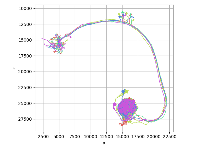
Let's demonstrate with a simple example using the default settings:
import navis
import matplotlib.pyplot as plt
nl = navis.example_neurons(kind="skeleton")
# Plot using default settings
fig, ax = navis.plot2d(nl, view=("x", "-z"), method="2d")
plt.tight_layout()
Note
We set view("x", "-z") above to get a frontal view of the example neurons. You may need to adjust this depending on the orientation of your neurons.
Above plot used the default matplotlib 2D plot. You might notice that the plot looks rather "flat" - i.e. neurons seem to be layered on top of each other without intertwining. That is one of the limitations of matplotlib's 3d backend. We can try to ameliorate this by adjusting the method parameter:
# Plot settings for more complex scenes - comes at a small performance cut though
fig, ax = navis.plot2d(nl, method="3d_complex", view=("x", "-z"))
plt.tight_layout()
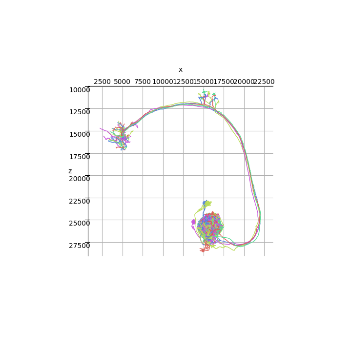
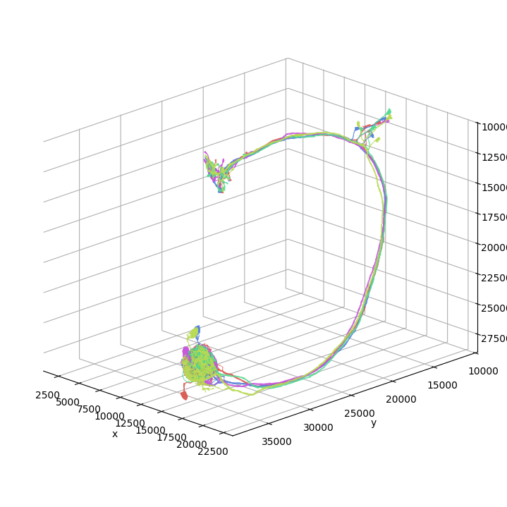
Looks better now, doesn't it? Now what if we wanted to adjust the perspective? For 3d axes, matplotlib lets us adjust the viewing angle by setting the elev, azim and roll attributes. See also this official explanation.
Let's give that a shot:
Plot again
fig, ax = nl.plot2d(
method="3d_complex", view=("x", "-z"), non_view_axes3d="show", radius=True
)
# Change view to see the neurons from a different angle
ax.elev = -20
ax.azim = 45
ax.roll = 180
plt.tight_layout()
Note
Did you note that we set non_view_axes3d='show' in above example? By default, NAVis hides the axis that is parallel to the viewing direction to not clutter the image. Because we were going to change the perspective, we set it to show. FYI: if the plot is rendered in a separate window (e.g. if you run Python from terminal), you can change the perspective by dragging the image.
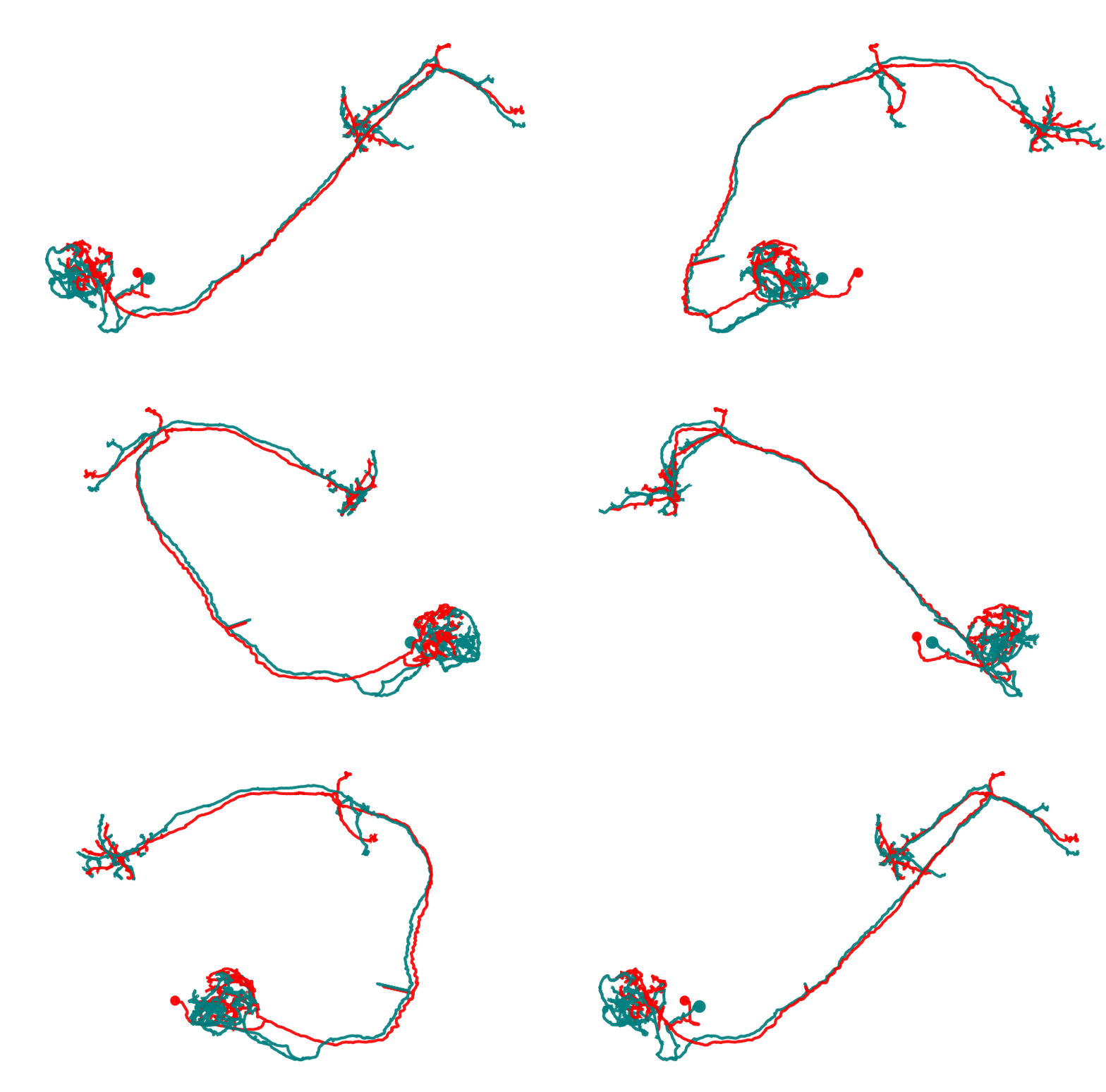
We can use this to generate small animations:
# Render 3D rotation
for i in range(0, 360, 10):
# Change rotation
ax.azim = i
# Save each incremental rotation as frame
plt.savefig('frame_{0}.png'.format(i), dpi=200)
3D plots#
By "3D plots" we typically mean interactive 3D plots as opposed to the (mostly) static 2D or semi-3D plots above. 3D plots are great for exploring your data interactively but you can also use them to generate high-quality static images.
As laid out at the top of this page: for 3D plots, we are using either octarine, plotly or k3d. In brief:
| backend | Jupyter | Terminal |
|---|---|---|
| octarine | yes | yes |
| plotly | yes | yes but only via export to html |
| k3d | yes | no |
By default, the choice is automatic and depends on (1) what backends are installed and (2) the context. The first available backend in each row wins:
| Context | Backend priority (first available wins) |
|---|---|
| IPython / Terminal / scripts | octarine plotly |
| Jupyter Lab / Notebook | plotly octarine k3d |
You can always force a specific backend using the backend parameter in navis.plot3d:
n = navis.example_neurons()
navis.plot3d(n)
n = navis.example_neurons()
navis.plot3d(n, backend='octarine')
n = navis.example_neurons()
navis.plot3d(n, backend='plotly')
n = navis.example_neurons()
navis.plot3d(n, backend='k3d')
Alternatively, you can also set the default backend using an environment variable. For example:
export NAVIS_PLOT3D_BACKEND="octarine"
Google Colaboratory
The jupyter_rfb that Octarine uses to render 3D plots in Jupyter does not work in Google Colaboratory. There, use the plotly backend instead.
With that out of the way, let's have a look at some 3D plots! You will notice that for the octarine and k3d backends we're just showing screenshots - that's because their interactive plots can't be embedded into this documentation.
Octarine#
Octarine works via a Viewer object which allows you to interactively add/remove objects, change colors, etc. It uses modern WGPU (rather than OpenGL) which makes it very fast even for large scenes:
nl = navis.example_neurons()
viewer = navis.plot3d(nl, backend='octarine')
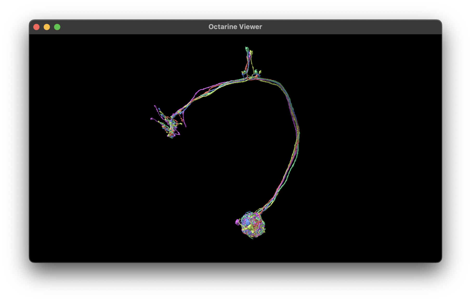
Showing the viewer in Jupyter
From Jupyter, you may need to call viewer.show() in the last line of the cell for the Octarine widget to appear.
A few things to know about the Octarine backend:
- The
vieweris dynamic - keep adding/removing items from other cells - but it dies with the kernel (unlikeplotly)! - NAVis tracks a "primary" viewer; subsequent
navis.plot3dcalls add to it. Force a new one withnavis.plot3d(nl, viewer='new')or target a specific one withnavis.plot3d(nl, viewer=viewer). - You can resize the canvas (in Jupyter by dragging the lower right corner).
- In Jupyter, rendering runs in your kernel and frames are streamed via a remote frame buffer (
jupyter_rfb); a remote kernel may add some lag.
Some important methods for the viewer object:
viewer.close() # (1)!
navis.close3d() # (2)!
navis.plot3d(nl) # (3)!
navis.plot3d(nl, viewer=viewer) # (4)!
viewer.clear3d() # (5)!
navis.clear3d() # (6)!
- Close the viewer.
- Close the current primary viewer.
- Add neurons to the primary viewer.
- Add neurons to a specific viewer.
- Clear the viewer.
- Clear the primary viewer.
The Octarine viewer has many more neat features - check out its documentation to learn more.
K3d#
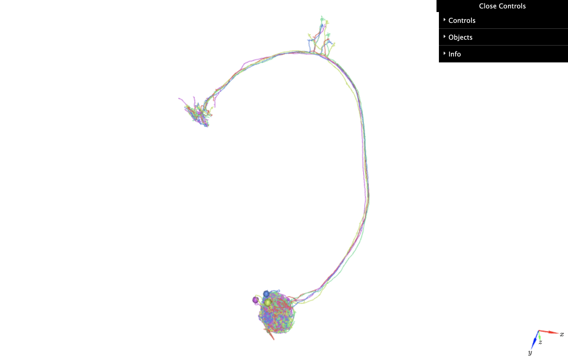
k3d plots work in Jupyter (and only there) but unlike plotly don't persist across sessions. Hence we will only briefly demo them using static screenshots and then move on to plotly. Almost everything you can do with the plotly backend can also be done with k3d (or octarine for that matter)!
p = navis.plot3d(nl, backend="k3d")
Plotly#
Last but not least, we have the plotly backend. This is the only backend which allows us to embed interactive 3D plots into this documentation. The main advantage of plotly is that it works "inline" in Jupyter notebooks and that you can export the plots as standalone HTML files. The main disadvantage is that it can be quite slow for large scenes and that the resulting .ipynb notebook files can get quite large.
Using plotly as backend generates "inline" plots by default (i.e. they are rendered right away):
navis.plot3d(
nl,
backend="plotly",
connectors=False,
radius=True, # use node radii for skeletons
legend_orientation="h", # horizontal legend (more space for plot)
)