Note
Click here to download the full example code
Normalizing Neurons#
Bring neurons into a canonical pose for machine-learning models.
NAVis ships a small navis.ml module with helpers for preparing neurons as model inputs. This first tutorial covers normalization; the sampling and augmentation tutorials cover the other two steps.
Note
These functions live under the navis.ml namespace (e.g. navis.ml.normalize_neuron) and are not lifted to the top level. See the Machine Learning API reference for the full list.
Why normalize?#
A neuron means the same thing no matter where it sits, how it is oriented or what units it was reconstructed in. A learning-based model should not have to spend capacity discovering that. navis.ml.normalize_neuron removes those nuisance degrees of freedom up front by mapping every neuron into a canonical frame with a single rigid-plus-uniform-scale transform:
- center (
c) moves a chosen reference point to the origin, - rotate (
R) aligns the principal axes of the arbor with x/y/z, and - scale (
s) normalizes the overall size.
Let's see it in action.
import navis
import numpy as np
import matplotlib.pyplot as plt

navis.config.pbar_hide = True

# Load an example skeleton (coordinates are in nanometers)
n = navis.example_neurons(1, kind="skeleton")

# Normalize its pose (defaults: center on centroid, PCA-orient, unit-RMS scale)
norm = navis.ml.normalize_neuron(n)
The transform is affine, so it is applied faithfully to everything the neuron carries - nodes/vertices, connectors, dotprops tangent vectors, radii and the .units - via navis.xform. The result is a copy; the input is never modified.
Let's check the two defining invariants: the normalized neuron is centered on the origin and has unit root-mean-square radius.
co = norm.nodes[["x", "y", "z"]].values
print("centroid :", co.mean(axis=0).round(6))          # ~ (0, 0, 0)
print("RMS radius:", round(float(np.sqrt((co ** 2).sum(axis=1).mean())), 6))  # ~ 1.0
Out:
centroid : [-0. -0.  0.]
RMS radius: 1.0
Note also how the units were rescaled to keep the physical size meaningful:
print("raw  units:", n.units)
print("norm units:", norm.units)
Out:
raw  units: 8 nanometer
norm units: 60.02434368177487 micrometer
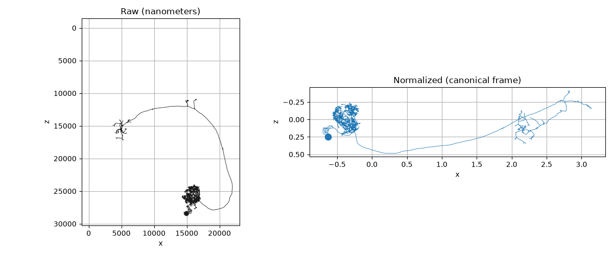
Let's visualize the raw vs. normalized neuron. Note the very different axis scales - nanometers on the left, dimensionless canonical units on the right - and that the normalized neuron is centered on the origin with its largest-variance axis along x.
fig, axes = plt.subplots(1, 2, figsize=(12, 5))

navis.plot2d(n, method="2d", view=("x", "-z"), ax=axes[0], color="k", lw=0.6)
navis.plot2d(norm, method="2d", view=("x", "-z"), ax=axes[1], color="C0", lw=0.6)

for ax in axes:
    ax.axhline(0, color="lightgrey", lw=0.5, zorder=0)
    ax.axvline(0, color="lightgrey", lw=0.5, zorder=0)
axes[0].set_title("Raw (nanometers)")
axes[1].set_title("Normalized (canonical frame)")
plt.tight_layout()
Pose invariance#
The whole point is that the canonical frame depends only on the shape, not on how the neuron happened to come in. Let's prove it: take the neuron, apply an arbitrary rotation and translation, then normalize both the original and the moved copy. They should land on top of each other.
# Build an arbitrary rigid transform (rotate ~50 deg about z, then translate)
theta = np.deg2rad(50)
M = np.eye(4)
M[:3, :3] = [
    [np.cos(theta), -np.sin(theta), 0],
    [np.sin(theta), np.cos(theta), 0],
    [0, 0, 1],
]
M[:3, 3] = [50_000, -30_000, 10_000]
moved = navis.xform(n, navis.transforms.AffineTransform(M))

# Normalize both and overlay
norm_a = navis.ml.normalize_neuron(n)
norm_b = navis.ml.normalize_neuron(moved)

fig, ax = plt.subplots(figsize=(6, 6))
navis.plot2d(norm_a, method="2d", view=("x", "-z"), ax=ax, color="C0", lw=1.5)
navis.plot2d(norm_b, method="2d", view=("x", "-z"), ax=ax, color="C1", lw=0.8, ls="--")
ax.set_title("Original (solid) vs. moved-then-normalized (dashed)")
plt.tight_layout()
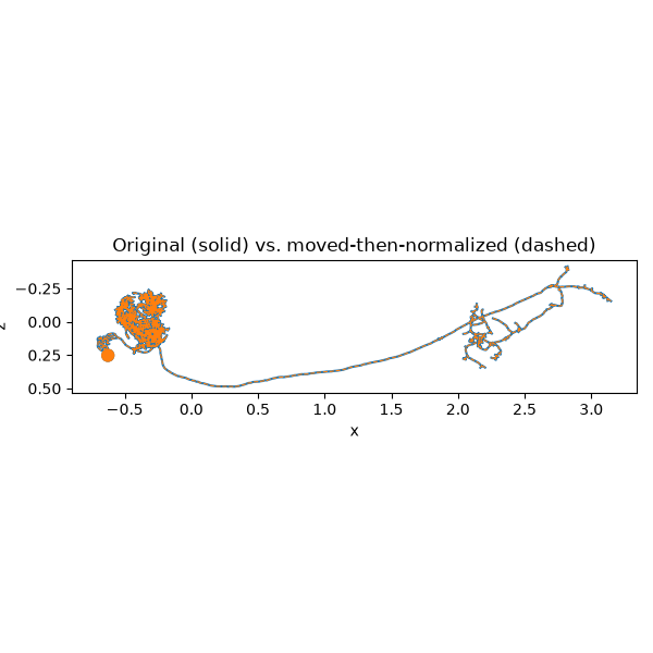
The two canonical poses are identical - the arbitrary rotation and translation were removed.
How PCA orientation is disambiguated
PCA orientation is disambiguated deterministically (the same shape always lands the same way up) and handedness is preserved - neurons are never mirrored, because morphology is chiral and a reflection would be a different shape. Orientation is unstable when two principal axes have near-equal spread (a neuron with no dominant axis).
The knobs#
Each of the three steps is configurable and can be turned off independently by passing None:
| Parameter | Options | Default | Effect |
|---|---|---|---|
center | "centroid", "bbox" (bounding-box midpoint), "soma", an explicit (x, y, z), None | "centroid" | moves the reference point to the origin |
rotate | "pca", None | "pca" | aligns the arbor's principal axes with x/y/z |
scale | "rms" (unit RMS radius), "extent" (longest axis becomes 1), "max" (farthest point becomes 1), None | "rms" | sets the overall size convention |
center picks the reference point moved to the origin - here the soma, with rotation and scaling switched off:
soma_centered = navis.ml.normalize_neuron(n, center="soma", rotate=None, scale=None)
sid = np.atleast_1d(n.soma)
soma_co = soma_centered.nodes.set_index("node_id").loc[sid, ["x", "y", "z"]].values
print("soma at origin:", np.allclose(soma_co.mean(axis=0), 0, atol=1e-5))
Out:
soma at origin: True
scale sets the size convention. The three options differ in what they hold fixed - "rms" is robust to a few far-flung nodes, while "max" gives a unit enclosing sphere:
for scale in ("rms", "extent", "max"):
    c = navis.ml.normalize_neuron(n, scale=scale).nodes[["x", "y", "z"]].values
    print(
        f"{scale:>7}: RMS={np.sqrt((c ** 2).sum(1).mean()):.3f}  "
        f"max_extent={(c.max(0) - c.min(0)).max():.3f}  "
        f"max_radius={np.sqrt((c ** 2).sum(1)).max():.3f}"
    )
Out:
    rms: RMS=1.000  max_extent=3.851  max_radius=3.254
 extent: RMS=0.260  max_extent=1.000  max_radius=0.845
    max: RMS=0.307  max_extent=1.183  max_radius=1.000
rotate is either "pca" (default) or None. Set scale=None to leave sizes (and radii and .units) untouched; set rotate=None to keep the incoming orientation. Passing center=None, rotate=None, scale=None is a no-op copy.
Mapping model outputs back#
Because normalization is a single matrix it is exactly invertible. Pass return_matrix=True to get the 4x4 homogeneous matrix - handy when a model predicts something in the normalized frame (a landmark, a direction, a denoised position) that you need back in the neuron's original coordinates.
norm, T = navis.ml.normalize_neuron(n, return_matrix=True)

# `T` maps original -> normalized; its inverse maps back.
pt_norm = norm.nodes[["x", "y", "z"]].values[0]             # a point in the model frame
pt_orig = (np.linalg.inv(T) @ np.append(pt_norm, 1))[:3]    # back to nanometers

print("recovered:", pt_orig.round(2))
print("original :", n.nodes[["x", "y", "z"]].values[0].round(2))
Out:
recovered: [15784. 37250. 28062.]
original : [15784. 37250. 28062.]
Whole populations#
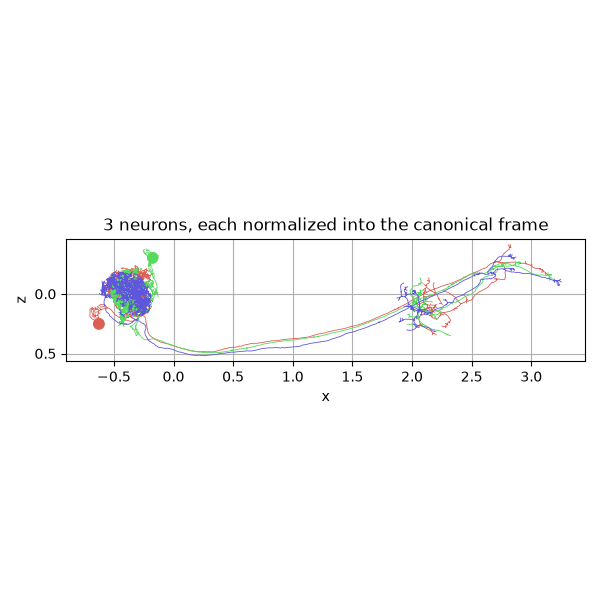
A navis.NeuronList is normalized element-wise - each neuron gets its own canonical frame, so a whole population lands in a shared, comparable coordinate system:
nl = navis.example_neurons(3, kind="skeleton")
nl_norm = navis.ml.normalize_neuron(nl)

fig, ax = plt.subplots(figsize=(6, 6))
navis.plot2d(nl_norm, method="2d", view=("x", "-z"), ax=ax, lw=0.6)
ax.set_title("3 neurons, each normalized into the canonical frame")
plt.tight_layout()
Tip
normalize_neuron also works on navis.MeshNeuron and navis.Dotprops (whose tangent vectors are rotated along with the points). VoxelNeurons are not supported - rotating a dense grid needs resampling; convert to points or a mesh first.
What's next#
A normalized neuron is still a variable-sized graph. The next tutorial turns it into a fixed-size model input:
- From Neurons to Model Inputs - sampling & chunking
- Augmenting Neurons - expanding a training set
See the Machine Learning API reference for the full list of functions.
Total running time of the script: ( 0 minutes 0.955 seconds)
Download Python source code: tutorial_ml_00_normalize.py