Neuron Topology#

Plot neurons as abstract topology graphs using several layout algorithms.

Skeletons in NAVis are hierarchical trees (hence the name TreeNeuron). As such they can be visualized as dendrograms or flat, graph-like plots using navis.plot_flat. This is useful to unravel otherwise complicated, overlapping branching patterns - e.g. when you want to show compartments or synapse positions within the neuron. Let's demo some layouts!

import navis
import matplotlib.pyplot as plt

# Load example neurons
nl = navis.example_neurons(n=4, kind="skeleton")

# Convert example neurons from voxels to nanometers
nl_nm = nl.convert_units("nm")

# Reroot to soma
nl_nm[nl_nm.soma != None].reroot(nl_nm[nl_nm.soma != None].soma, inplace=True)

Available layouts#

navis.plot_flat supports one native layout (subway) plus a family of graphviz layouts. For graphviz layouts the engine name matches the layout name:

Layout	Graphviz engine	Notes
`subway`	— (native)	Preserves branch lengths; great for side-by-side comparisons
`dot`	`dot`	Dendrogram; preserves branch lengths
`twopi`	`twopi`	Radial dendrogram; preserves branch lengths
`neato`	`neato`	Force-directed; can be slow - downsample first
`fdp`	`fdp`	Force-directed; can be slow - downsample first
`sfdp`	`sfdp`	Force-directed; scalable variant

Graphviz layouts need pygraphviz

Every layout except subway needs pygraphviz and the underlying graphviz library installed. Install pygraphviz with:

pip install pygraphviz

For details on the layouts, see the graphviz docs.

The call is the same for every layout - just swap the layout argument:

subwaydottwopineatofdpsfdp

navis.plot_flat(nl_nm[0], layout="subway", connectors=True)

navis.plot_flat(nl_nm[0], layout="dot", connectors=True, color="k")

navis.plot_flat(nl_nm[0], layout="twopi", connectors=True, color="k")

# neato can be expensive - downsample the neuron first
ds = navis.downsample_neuron(nl_nm[0], 10, preserve_nodes="connectors")
navis.plot_flat(ds, layout="neato", connectors=True, color="k")

ds = navis.downsample_neuron(nl_nm[0], 10, preserve_nodes="connectors")
navis.plot_flat(ds, layout="fdp", connectors=True, color="k")

navis.plot_flat(nl_nm[0], layout="sfdp", connectors=True, color="k")

Subway maps#

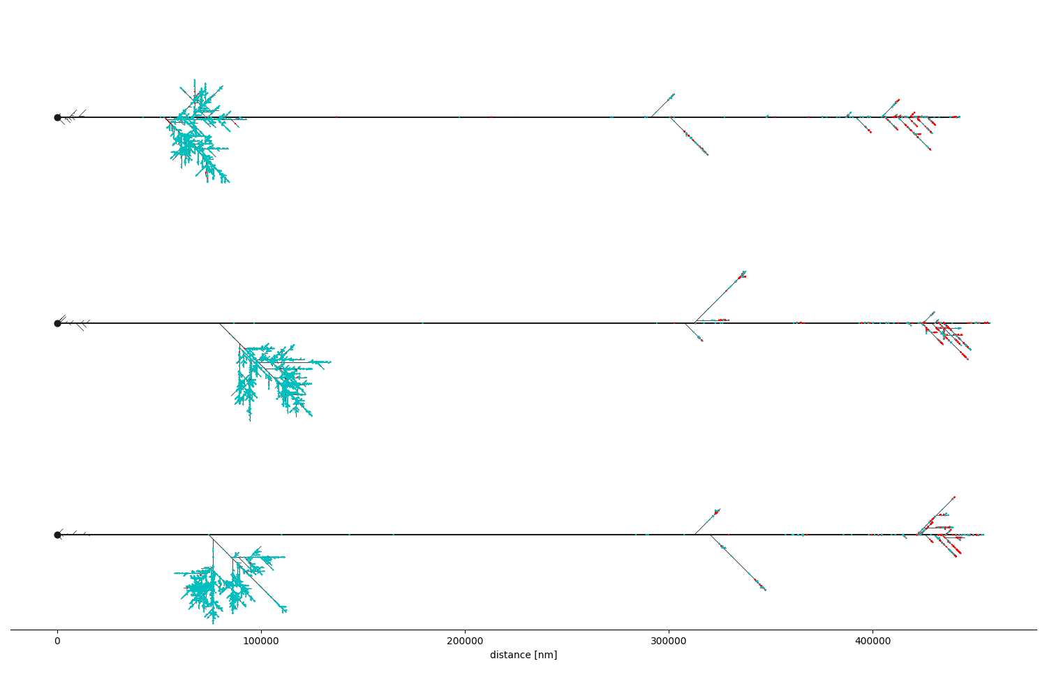
The subway layout is native (no graphviz needed) and is nice for side-by-side comparisons of neurons. Let's render it for a few of ours:

# Generate one axis for each neuron
fig, axes = plt.subplots(3, 1, figsize=(15, 10), sharex=True)

navis.plot_flat(nl_nm[0], layout="subway", connectors=True, ax=axes[0])
navis.plot_flat(nl_nm[1], layout="subway", connectors=True, ax=axes[1])
navis.plot_flat(nl_nm[3], layout="subway", connectors=True, ax=axes[2])

# Clean up the axes
for ax in axes[:-1]:
    ax.set_axis_off()

for sp in ["left", "right", "top"]:
    axes[-1].spines[sp].set_visible(False)
axes[-1].set_yticks([])

_ = axes[-1].set_xlabel("distance [nm]")
plt.tight_layout()

Highlighting connectors#

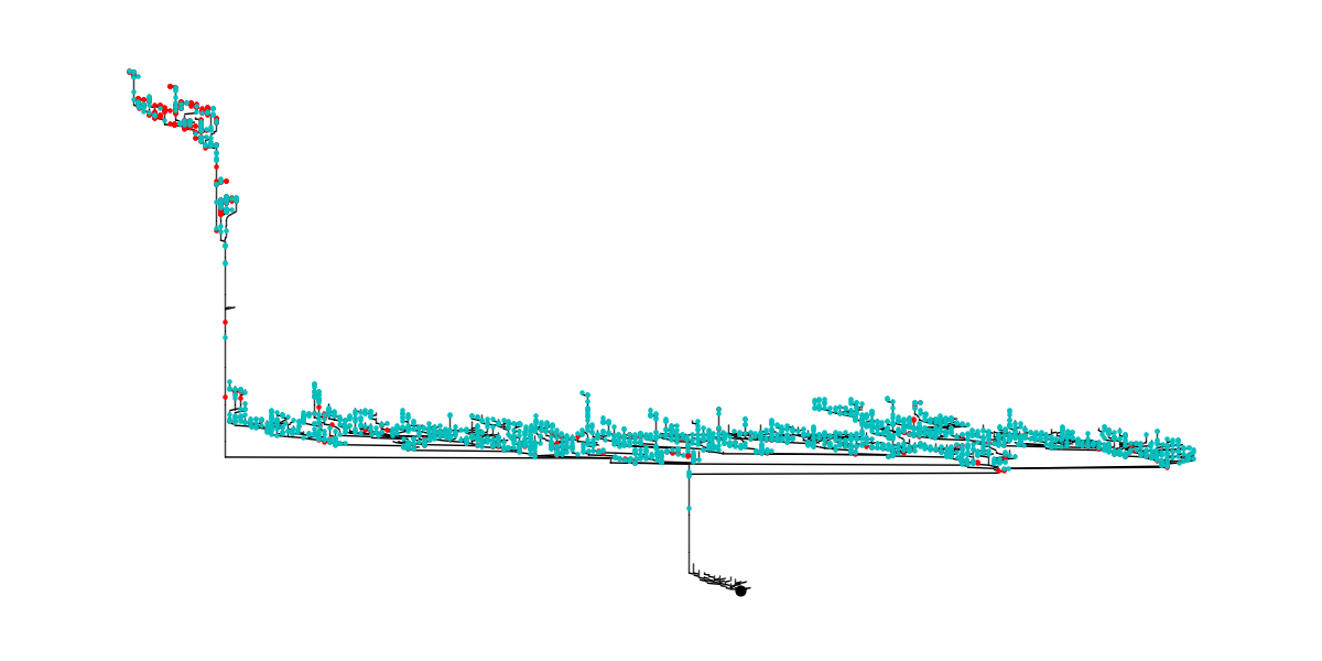
For any layout you can highlight specific connectors by their ID. Here we highlight the first 100 on a dot layout:

n = nl_nm[0]
highlight = n.connectors.connector_id[:100]

ax = navis.plot_flat(
    n,
    layout="dot",
    highlight_connectors=highlight,
    color="k",
    syn_marker_size=2,
)
plt.tight_layout()

Total running time of the script: ( 0 minutes 5.689 seconds)

Download Python source code: tutorial_plotting_03_dend.py

Download Jupyter notebook: tutorial_plotting_03_dend.ipynb

Gallery generated by mkdocs-gallery