Note
Click here to download the full example code
From Neurons to Model Inputs#
Turn neurons into fixed-size model inputs: feature point clouds and batchable patches.
Neurons are variable-sized graphs and meshes with uneven node/vertex density. Most models want a fixed number of points, sampled evenly and at a controlled resolution. The navis.ml toolkit answers three separate questions:
- Where do the points come from? The cable of a skeleton, the surface of a mesh, or an existing point cloud.
- How many / how dense? A fixed count (
n_points), a fixed resolution (density), or a fixed inter-point distance (spacing) - see the next section. - One cloud per neuron, or many patches? Sample the whole neuron, or tile it into fixed-size fragments/patches.
| Function | Input | What you get |
|---|---|---|
navis.sample_skeleton | skeleton | equal-spacing points, deterministic, coordinates only |
navis.ml.sample_cable | skeleton | stratified arclength points + interpolated features |
navis.ml.sample_surface | mesh | area-weighted surface points + per-vertex features |
navis.ml.sample_points_uniform | point cloud | an evenly-spread subsample |
navis.ml.estimate_spacing | point cloud | the measured spacing/density (the inverse of the knobs) |
navis.ml.chunk_neuron | skeleton or mesh | fixed-size fragments of existing points (indices) |
navis.ml.sample_patches | skeleton or mesh | resample at a density, then tile into fixed-size patches |
Note
This tutorial follows on from Normalizing Neurons. In practice you would usually normalize before sampling so every cloud lives in the same canonical frame - and so density/spacing are expressed in that frame's units.
import navis
import numpy as np
import matplotlib.pyplot as plt

navis.config.pbar_hide = True

n = navis.example_neurons(1, kind="skeleton")
m = navis.example_neurons(1, kind="mesh")
One dial, three faces: n_points, density, spacing#
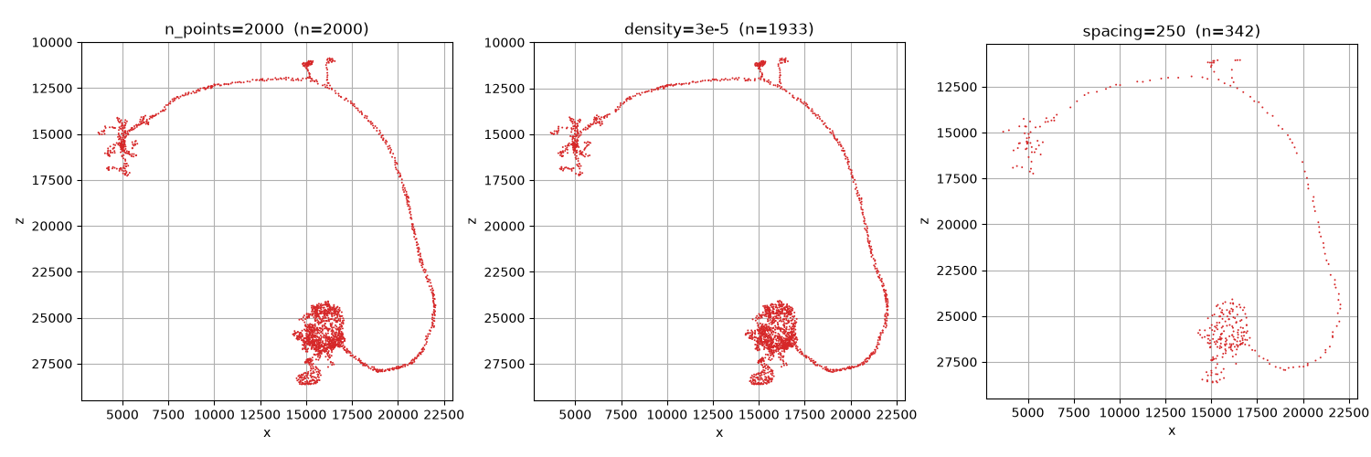
A neuron's size ties together how many points you draw and how far apart they are, so you can pin exactly one of these three (the samplers reject more than one). They are shared by navis.sample_skeleton, navis.ml.sample_cable and navis.ml.sample_surface:
Draw the same number of points from every neuron. The resolution then varies with size: a large arbor is sampled sparsely, a small one densely.
Use when the model needs fixed-size inputs (e.g. a 1024-point tensor).
navis.ml.sample_cable(n, n_points=1000)
navis.ml.sample_surface(m, n_points=2000)
Draw a fixed number of points per unit cable length (skeleton) or surface area (mesh); the count scales with neuron size.
Use when local neighbourhoods must mean the same physical scale across neurons - exactly what k-NN / ball-query models (PointNet++, DGCNN, point transformers) assume.
navis.ml.sample_cable(n, density=5e-3)     # points per unit length
navis.ml.sample_surface(m, density=3e-5)   # points per unit area
Fix the distance between neighbouring points. For a skeleton this is the exact step along the cable; for a mesh it is a Poisson-disk minimum distance, so the count comes out of rejection sampling and may vary.
Related to density by density ~ 1 / spacing (cable) or ~ 1 / spacing**2 (surface).
navis.ml.sample_cable(n, spacing=250)      # distance between samples
navis.ml.sample_surface(m, spacing=200)    # mode="even" only
Here are all three on the mesh surface. n_points fixes the count; density and spacing fix the resolution and let the count fall out:
by_count = navis.ml.sample_surface(m, n_points=2000, random_state=0)
by_density = navis.ml.sample_surface(m, density=3e-5, random_state=0)
by_spacing = navis.ml.sample_surface(m, spacing=250, random_state=0)

fig, axes = plt.subplots(1, 3, figsize=(15, 5))
for ax, s, title in zip(
    axes,
    (by_count, by_density, by_spacing),
    (f"n_points=2000  (n={len(by_count)})",
     f"density=3e-5  (n={len(by_density)})",
     f"spacing=250  (n={len(by_spacing)})"),
):
    navis.plot2d(s[["x", "y", "z"]].values, method="2d", view=("x", "-z"),
                 ax=ax, scatter_kws=dict(c="C3", s=2))
    ax.set_title(title)
plt.tight_layout()
Sampling a skeleton: sample_cable#
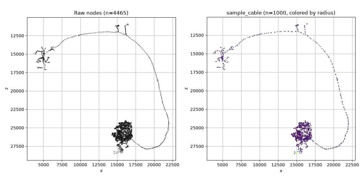
Skeleton nodes are rarely spaced evenly along the cable, so drawing nodes at random over-weights densely-noded regions. navis.ml.sample_cable instead samples points at uniform arclength along the edges and interpolates node attributes onto each sample. Draws are stratified (one jittered sample per equal-measure bin) for exactly even coverage.
pts = navis.ml.sample_cable(n, n_points=1000, interpolate="radius", random_state=0)
pts.head()
You get back a tidy DataFrame with the sampled coordinates, the requested interpolated columns, and a source_id recording which node each sample came from (join it to pull in any other per-node attribute):
print(list(pts.columns))
Out:
['x', 'y', 'z', 'radius', 'source_id']
Let's compare the raw nodes (density tracks the reconstruction) against the arclength-uniform sample (density tracks the cable). Point size encodes the interpolated radius.
fig, axes = plt.subplots(1, 2, figsize=(12, 6))

navis.plot2d(
    n.nodes[["x", "y", "z"]].values, method="2d", view=("x", "-z"),
    ax=axes[0], scatter_kws=dict(c="k", s=2),
)
axes[0].set_title(f"Raw nodes (n={n.n_nodes})")

navis.plot2d(
    pts[["x", "y", "z"]].values, method="2d", view=("x", "-z"),
    ax=axes[1], scatter_kws=dict(c=pts["radius"].values, s=4, cmap="viridis"),
)
axes[1].set_title("sample_cable (n=1000, colored by radius)")
plt.tight_layout()
The same neuron sampled by density or spacing gives a count that tracks its cable length instead:
for kw in (dict(n_points=1000), dict(density=5e-3), dict(spacing=250)):
    out = navis.ml.sample_cable(n, **kw, random_state=0)
    print(f"{kw} -> {len(out)} points")
Out:
{'n_points': 1000} -> 1000 points
{'density': 0.005} -> 1332 points
{'spacing': 250} -> 1066 points
Tip
Pass weights="radius" to bias sampling towards thicker cable (a lateral-surface-area-like weighting), or interpolate=True to attach every non-structural node column.
sample_cable vs sample_skeleton#
There are two ways to turn a skeleton into points; pick by whether you need features and randomness:
Stratified (randomised) arclength sampling. Interpolates radius/other columns onto each point and records source_id. Returns a DataFrame. The richer, ML-facing sampler - use it to build feature clouds.
Deterministic equal-spacing sampling: the same points every call, coordinates only (no attributes). Returns a plain (n, 3) array. Use it when you want a reproducible geometric skeletonisation without features.
navis.sample_skeleton(n, n_points=1000) # or density= / spacing=
Sampling a mesh: sample_surface#
Mesh vertex density tracks surface detail, not the arbor, so meshes are best sampled by surface area. navis.ml.sample_surface does area-weighted (blue-noise) sampling and, like sample_cable, records each sample's source vertex so per-vertex labels transfer onto the cloud.
Per-vertex attributes ride along via the attributes argument - here we fake a per-vertex label and transfer it onto the sampled points:
label = (m.vertices[:, 2] > np.median(m.vertices[:, 2])).astype(int)
surf = navis.ml.sample_surface(m, n_points=2000, attributes={"label": label}, random_state=0)
print(surf["label"].value_counts().to_dict())
Out:
{1: 1017, 0: 983}
Note
mode="even" (the default) is blue-noise sampling; mode="surface" is plain area-weighted random sampling; mode="vertex" draws existing vertices. Only "even" supports spacing (it is the Poisson-disk minimum distance).
Measuring resolution: estimate_spacing#
navis.ml.estimate_spacing is the inverse of the spacing/density knobs: give it any cloud and it reports the characteristic nearest-neighbour distance. Use it to audit a cloud, or to pick a density/spacing for a whole dataset.
print("cable sample  :", round(navis.ml.estimate_spacing(pts[["x", "y", "z"]].values), 1))
print("surface sample:", round(navis.ml.estimate_spacing(surf[["x", "y", "z"]].values), 1))
Out:
cable sample  : 117.3
surface sample: 112.8
Subsampling a cloud: sample_points_uniform#
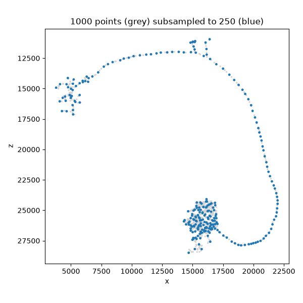
If you already have a point cloud (e.g. dotprops points, or the output of the samplers above) and just want fewer, evenly-spread points, navis.ml.sample_points_uniform subsamples it. It uses farthest-point sampling for the most uniform coverage, falling back to a cheaper decimation on large clouds (method="auto").
cloud = pts[["x", "y", "z"]].values                 # the 1000-point cable sample
sub = navis.ml.sample_points_uniform(cloud, size=250)

fig, ax = plt.subplots(figsize=(6, 6))
navis.plot2d(cloud, method="2d", view=("x", "-z"), ax=ax, scatter_kws=dict(c="lightgrey", s=6))
navis.plot2d(sub, method="2d", view=("x", "-z"), ax=ax, scatter_kws=dict(c="C0", s=12))
ax.set_title("1000 points (grey) subsampled to 250 (blue)")
plt.tight_layout()
Tip
Use output="indices" or output="mask" to get the selection rather than the points - handy for subsetting a matching feature array in lock-step.
Chunking into fixed-size fragments: chunk_neuron#
Instead of one cloud per neuron, you sometimes want to tile a neuron into many fixed-size fragments - e.g. to make per-fragment predictions. navis.ml.chunk_neuron returns a list of positional index arrays, each addressing rows of x.nodes (skeleton) or x.vertices (mesh). It tiles the neuron's existing points; it does not resample, so it has no density control (see sample_patches below for that).
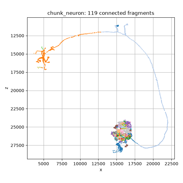
By default fragments grow along the arbor (geodesic distance), so each one is a connected piece:
chunks = navis.ml.chunk_neuron(n, size=300, mode="partition", undersized="keep")
print(f"{len(chunks)} fragments")

co = n.nodes[["x", "y", "z"]].values
fig, ax = plt.subplots(figsize=(6, 6))
cmap = plt.get_cmap("tab20")
for i, ch in enumerate(chunks):
    real = ch[ch >= 0]                              # drop any pad slots (see below)
    navis.plot2d(
        co[real], method="2d", view=("x", "-z"),
        ax=ax, scatter_kws=dict(c=[cmap(i % 20)], s=4),
    )
ax.set_title(f"chunk_neuron: {len(chunks)} connected fragments")
plt.tight_layout()
Out:
119 fragments
For a stackable batch, keep the default undersized="pad": every fragment is padded up to size with a pad token (default -1) so they stack into one array.
chunks = navis.ml.chunk_neuron(n, size=256, mode="partition")   # undersized="pad"
batch = np.stack(chunks)
print("batch shape:", batch.shape)                              # (n_fragments, 256)
Out:
batch shape: (123, 256)
Warning
Don't index coordinates with a padded fragment directly - a negative pad value is a valid (wrong) index and silently returns real rows. Mask first:
real = chunk[chunk >= 0]          # drop pad slots
patch = co[real]                  # (<= size, 3)
node_ids = n.nodes.node_id.values[real]
chunk_neuron has four modes; the first two emerge a fragment count, the last two let you set it via k / sampling_factor:
Non-overlapping tiles covering every point once (the default). The remainder that can't fill a whole tile is handled per undersized.
Overlapping tiles that cover every point at least once - tiles may reuse points to stay full-size.
k (or sampling_factor x) fragments from random seeds. Good for oversampling a training set.
Like random, but seeds are evenly spread by farthest-point sampling (deterministic unless you pass random_state). Good for even oversampling.
connected=False grows fragments by Euclidean distance instead (the size nearest points in space), which packs tightly but ignores the arbor.
spaced = navis.ml.chunk_neuron(n, size=200, mode="spaced", k=6, random_state=0)
print(f"{len(spaced)} evenly-spaced fragments of {[len(c) for c in spaced]} nodes")
Out:
6 evenly-spaced fragments of [200, 200, 200, 200, 200, 200] nodes
Patches at a controlled resolution: sample_patches#
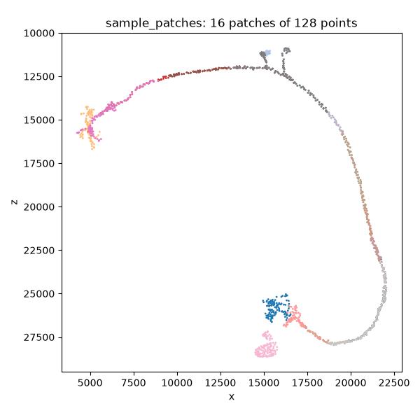
chunk_neuron tiles existing points, so a fragment's density is whatever the reconstruction had. When you want fixed-size patches and a fixed resolution - the standard "group K points within radius r" input for point-cloud models - use navis.ml.sample_patches. It resamples the neuron to a uniform cloud at your density/spacing (via sample_surface/sample_cable) and then tiles that cloud into n_points-sized spatial patches.
Because the cloud is uniform, n_points + density pin each patch's physical extent - and that extent is the same across patches and across neurons.
The result is one tidy DataFrame with a chunk_id column (overlapping patches simply repeat a point's row under each patch it belongs to):
patches = navis.ml.sample_patches(
    m, n_points=128, density=3e-5, mode="spaced", random_state=0
)
print(f"{patches.chunk_id.nunique()} patches, {len(patches)} rows total")
print(list(patches.columns))

fig, ax = plt.subplots(figsize=(6, 6))
for cid, g in patches.groupby("chunk_id"):
    navis.plot2d(
        g[["x", "y", "z"]].values, method="2d", view=("x", "-z"),
        ax=ax, scatter_kws=dict(c=[cmap(cid % 20)], s=4),
    )
ax.set_title(f"sample_patches: {patches.chunk_id.nunique()} patches of 128 points")
plt.tight_layout()
Out:
16 patches, 2048 rows total
['x', 'y', 'z', 'source_id', 'face', 'chunk_id']
groupby("chunk_id") gives you the patches; stack them into a batch tensor:
batch = np.stack([g[["x", "y", "z"]].values for _, g in patches.groupby("chunk_id")])
print("patch batch:", batch.shape)                  # (n_patches, 128, 3)
Out:
patch batch: (16, 128, 3)
Foveated patches: detail and context#
A uniform patch spends its whole budget at one resolution, so n_points fixes the detail and the extent: ask for fine detail and the patch sees only a sliver of neurite; ask for context and the detail is gone. Your eye solves this with a fovea - sharp in the centre, coarse in the periphery - and foveate=True does the same, thinning the point density outwards from the patch centre.
| Knob | What it does |
|---|---|
foveate | None | True - off, or scale-free thinning. A float applies a literal 1 / r**foveate falloff instead |
reach | How far the periphery extends: the patch grows reach * n_points candidates, then thins back down |
fovea | Keep the innermost fovea points at full density before the falloff starts - widens the chunk_focus == 1 core |
Same 128 points in both panels - the foveated one keeps the dense core and spends what's left following the axon all the way back to the soma:
kw = dict(n_points=128, density=3e-5, mode="spaced", k=1, random_state=1)
uniform_patch = navis.ml.sample_patches(m, **kw)
fov_patch = navis.ml.sample_patches(m, foveate=True, reach=32, **kw)


def span(d):
    """Furthest any point in the patch sits from its seed (the first row)."""
    co = d[["x", "y", "z"]].values
    return np.linalg.norm(co - co[0], axis=1).max()


fig, axes = plt.subplots(1, 2, figsize=(10, 5))
for ax, d, title in [(axes[0], uniform_patch, "uniform"), (axes[1], fov_patch, "foveated")]:
    navis.plot2d(m, method="2d", view=("x", "-z"), ax=ax, color=(0.9, 0.9, 0.9))
    navis.plot2d(
        d[["x", "y", "z"]].values, method="2d", view=("x", "-z"), ax=ax,
        scatter_kws=dict(c=d.get("chunk_dist", np.zeros(len(d))), cmap="viridis", s=12),
    )
    ax.set_title(f"{title}: 128 points, span {span(d):.0f}")
plt.tight_layout()
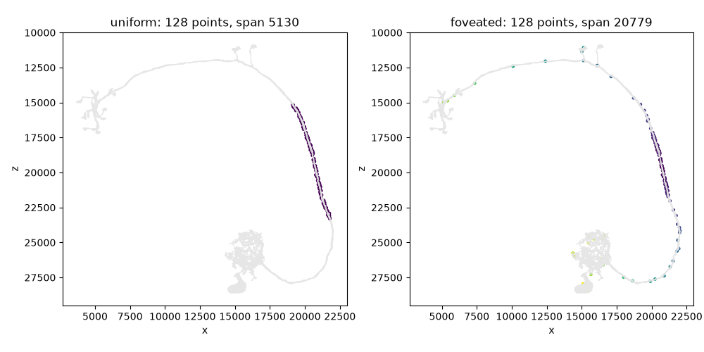
Foveated patches carry two extra columns, and a model wants both - a foveated patch spans orders of magnitude in radius and in local resolution, neither of which is recoverable from the raw coordinates:
| Column | Meaning |
|---|---|
chunk_dist | distance to the patch's seed (geodesic when connected=True) - the radial coordinate |
chunk_focus | how "in focus" the point is: 1.0 at full density, falling towards 0 where the cloud was thinned |
chunk_focus is the fraction of the cloud kept around each point, so it doubles as a per-point confidence weight - and thresholding it pulls out just the crisp core:
print(f"reach: {span(fov_patch) / span(uniform_patch):.0f}x the uniform patch")
print(f"core:  {(fov_patch.chunk_dist <= span(uniform_patch)).sum()}/128 points still "
      "inside the uniform patch's radius")

in_focus = fov_patch[fov_patch.chunk_focus == 1.0]
print(f"focus: {len(in_focus)}/128 points at full density, out to "
      f"{in_focus.chunk_dist.max():.0f} of {fov_patch.chunk_dist.max():.0f}")
print(f"       falls to {fov_patch.chunk_focus.min():.4f} at the rim "
      f"(~1 point kept in {1 / fov_patch.chunk_focus.min():.0f})")
Out:
reach: 4x the uniform patch
core:  82/128 points still inside the uniform patch's radius
focus: 73/128 points at full density, out to 2863 of 27036
       falls to 0.0098 at the rim (~1 point kept in 102)
That is the whole trade, and it is a logarithmic one: each 4x of reach costs only a handful of core points, because the thinning places roughly equal points per octave of radius. Raise density (or n_points) if you need the core back at full resolution.
navis.ml.sample_patches(m, n_points=128, density=3e-5,
                        foveate=True, reach=32)
Points are spaced geometrically in radial rank. Since a point's rank is the number of cloud points closer than it, this is a 1 / r**D falloff for a locally D-dimensional cloud - without ever measuring D. Prefer it: D really does run from ~1 on a thin neurite to ~2 on a soma within a single mesh, so it self-calibrates per patch.
navis.ml.sample_patches(m, n_points=128, density=3e-5,
                        foveate=2.0, reach=32)
A true 1 / r**2 weighting keyed on distance. Use it when you want that exact physical density and accept that the core/periphery split then shifts with the local geometry.
navis.ml.sample_patches(m, n_points=128, density=3e-5,
                        foveate=True, reach=32, fovea=32)
The innermost 32 points are taken at full cloud density before any thinning, for a genuinely crisp core; the remaining 96 spread out over the periphery.
Foveated patches do not tile
They deliberately overlap, so foveate requires mode="spaced" or mode="random" and raises on "partition"/"cover" - neither the disjoint nor the full-coverage guarantee can hold when a patch samples only a fraction of the territory it spans.
Cost
reach is the cost knob: growth does reach x n_points work per patch, while the thinning itself is free. reach=None reaches over the whole connected component - useful, but pay for it deliberately.
A typical pipeline#
Putting it together, a common recipe for feeding a batch of skeletons to a point-cloud model is: normalize -> sample -> stack. Sampling by density here would instead give every neuron the same resolution (and a variable count).
nl = navis.example_neurons(3, kind="skeleton")

batch = np.stack([
    navis.ml.sample_cable(
        navis.ml.normalize_neuron(nrn),     # canonical frame (tutorial 00)
        n_points=1024, random_state=0,
    )[["x", "y", "z"]].values
    for nrn in nl
])
print("model input batch:", batch.shape)    # (n_neurons, 1024, 3)
Out:
model input batch: (3, 1024, 3)
What's next#
- Normalizing Neurons - the canonical-pose step that usually comes first.
- Augmenting Neurons - expand a training set with realistic perturbations.
See the Machine Learning API reference for the full list of functions.
Total running time of the script: ( 0 minutes 2.699 seconds)
Download Python source code: tutorial_ml_01_sampling.py