Label Propagation#

Spread a sparse set of labels across a neuron using its topology.

One of the most intuitive applications for this is to try to label the axon and dendrite of a neuron based on the distribution of pre- and postsynapses alone.

Background#

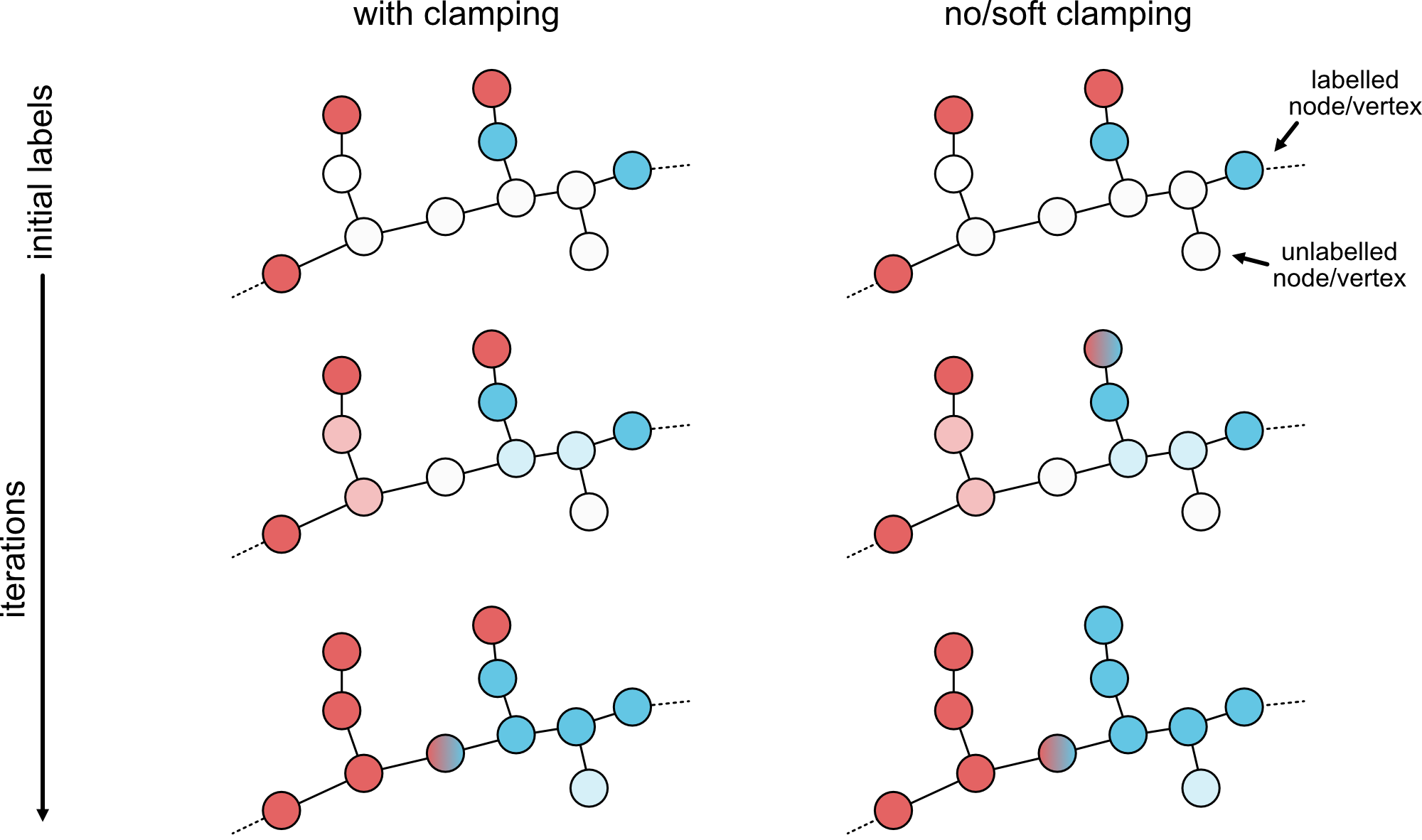
The function that does the heavy lifting is navis.propagate_labels(). It takes a neuron (skeleton or mesh) plus a set of initial labels and spreads those labels across the neuron following its topology.

How propagation works (the math)

Propagation is implemented as a series of matrix multiplications. The neuron's topology - node-to-node for skeletons, vertex-to-vertex for meshes - is an adjacency matrix, and the labels are a vector. Multiplying the two spreads the labels one step across the neuron; repeating the operation carries them further. We iterate until the labels stop changing (tol) or a maximum number of iterations is reached (max_iter).

graph LR
    A["Adjacency matrix<br>(topology)"] --> X(("×"))
    L["Label vector"] --> X
    X --> U["Updated labels"]
    U -->|"repeat until tol / max_iter"| X

The propagation can be tuned with a few knobs:

Parameter	What it controls
`weights`	Per-label importance as a `dict` mapping label → float. Higher-weighted labels propagate more readily; `None` (default) treats all labels equally.
`clamping`	Whether the initial labels may change. `True` (default) keeps them fixed; `False` lets them change freely; `"soft"` / `"soft:alpha"` lets them change but biases them toward their original value.
`tol`	Convergence tolerance. With the default (`>= 1`) we stop once no label has flipped for `tol` iterations; values `< 1` compare probability changes instead.
`max_iter`	Maximum number of iterations.

Axon-Dendrite Labeling#

To demonstrate label propagation, we will create labels from its pre- and postsynapses, and propagate those labels across the neuron to try to label the axon and dendrite.

import navis

import numpy as np
import pandas as pd
import seaborn as sns
import matplotlib.pyplot as plt


sns.set_color_codes("muted")

# Load the example neuron. This is a mesh but the same process works for skeletons as well.
n = navis.example_neurons(1, kind='mesh')

First, we need to collect our initial sets of labels. There are various options but here we will create a vector that, for each vertex in the mesh, says whether it contains pre- or postsynapses.

# Snap each pre/postsynapses to the closest vertex
pre_vertices, _ = n.snap(n.presynapses[['x', 'y', 'z']].values)
post_vertices, _ = n.snap(n.postsynapses[['x', 'y', 'z']].values)

# Create an empty vector of labels
labels = np.full(n.n_vertices, fill_value=np.nan, dtype=object)

# Fill in the labels for the pre- and postsynapses
labels[post_vertices] = 'post'
labels[pre_vertices] = 'pre'
# Note that if a vertex contains both pre- and postsynapses, it will be labeled as 'pre' because we overwrite the 'post' label.
# There are more clever ways to handle this (e.g. using weights) but here we'll keep it simple.

# Check the distribution of our initial labels
np.unique(labels.astype(str), return_counts=True)

Out:

(array(['nan', 'post', 'pre'], dtype='<U4'), array([4298, 1457,  554]))

With our initial labels ready, we can propagate them. By default the initial labels are "clamped" (fixed). But in insect neurons pre- and postsynapses are mixed - the axon carries some postsynapses and vice versa - so for a smooth labeling we let the initial labels change too, via clamping=False (or a soft clamp like clamping="soft:0.9"; see the table above).

pred = navis.propagate_labels(n, labels, clamping=False, max_iter=10000, tol=1e-6, verbose=True)

Out:

Finished 10,000 iterations without convergence (last largest change: 1.18e-05).

Note how the prediction didn't converge? Worst case, that means some vertices are never reached and stay unlabeled; here it just means the probabilities haven't fully stabilised yet - which may not even change the final labels. Raise max_iter (or lower tol) for a fully converged solution, trading runtime for convergence.

Let's check the distribution of our predicted labels:

np.unique(pred.astype(str), return_counts=True)

Out:

(array(['nan', 'post', 'pre'], dtype='<U4'), array([ 164, 4437, 1708]))

So we seem to be having some None values in our predictions. On closer inspection, these are little internal "flakes" that are disconnected from the rest of the neuron mesh and thus never receive any signal during the propagation. We will ignore those for now!

Next, we will visualise the predicted labels across the neuron.

# Fill the Nones with a new category for plotting
pred[pd.isnull(pred)] = "unlabeled"

navis.plot3d(
    n,
    color_by=pred,
    palette={"pre": "red", "post": "cyan", "unlabeled": "lightgray"},
    backend="plotly",
)

That doesn't look too bad! But we can do even better: our pred vector is effectively a hard assignment of each vertex to a single label, but the underlying propagation process actually gives us probabilities for each label at each vertex. We can use those probabilities to get a more nuanced view of the predicted labels across the neuron.

pred, prob, order = navis.propagate_labels(n, labels, clamping=False, max_iter=10000, tol=1e-6, verbose=True, return_probs=True)

# `order` gives us the order of labels in the `prob` array
print("Label order:", order)

# Inspect probability vector
prob

Out:

Finished 10,000 iterations without convergence (last largest change: 1.18e-05).
Label order: ['post', 'pre']

array([[0.84158283, 0.15841714],
       [0.83607066, 0.16392933],
       [0.83609617, 0.16390383],
       ...,
       [0.        , 0.        ],
       [0.23121291, 0.7687871 ],
       [0.23119102, 0.76880896]], shape=(6309, 2), dtype=float32)

Let's visualise the probabilities for the "post" label across the neuron:

navis.plot3d(
    n,
    color_by=prob[:, 0],
    palette="coolwarm",
    backend="plotly",
)

As you can see, the probability for "post" decreases (red -> blue) as we move from the proximal dendrites to the distal axon - which is exactly what we would expect! If you wanted, you could use those probabilities to make finer categories such low vs high confidence axon/dendrite labels, or even just use the probabilities directly for downstream analyses instead of hard labels.

Notes#

Note

If your neuron isn't contiguous (i.e. has multiple disconnected components), labels can't propagate across the gaps.
Propagating across a large mesh can be computationally expensive - downsampling the neuron first is a good way to speed things up.

Axon-dendrite splits

A deep dive into determining axon vs dendrite, including alternative flow-based approaches.

Axon-dendrite tutorial

Total running time of the script: ( 0 minutes 3.081 seconds)

Download Python source code: tutorial_morpho_02_label_prop.py

Download Jupyter notebook: tutorial_morpho_02_label_prop.ipynb

Gallery generated by mkdocs-gallery