Note
Click here to download the full example code
IVSCC morphometrics#
Measure cortical neurons compartment by compartment.
This example is not executed
Like the skeleton QC tutorial, this one is not run when the docs are built - it pulls ~25 reconstructions from a remote repository, which is not something to lean on in CI. The code is real and runnable; the outputs and plots shown here are statically embedded.
Most morphometrics treat a neuron as one undifferentiated tree. For a cortical neuron that throws away the most informative thing about it: a layer-5 pyramidal cell is not "a tree with 800 µm of reach", it is a basal bush around the soma, an apical trunk climbing to the pia, and an axon heading the other way. The three answer different questions and have to be measured separately.
navis.ivscc_features does exactly that. It follows the feature set from the Allen Institute's IVSCC pipeline: split the neuron on its compartment labels, measure each part on its own, then add a handful of features describing how the parts relate to the soma and to each other.
graph LR
    A[Labelled<br>skeleton] -->|"label = 2, 3, 4"| B[axon<br>basal dendrite<br>apical dendrite];
    B --> C[per-compartment<br>size, topology, shape];
    B --> D[between-compartment<br>depth overlap];
    A --> E[whole-cell<br>soma features];
    C --> F[one row<br>per neuron];
    D --> F;
    E --> F;
Requirements
This tutorial fetches reconstructions from the Brain Image Library over the network - no account or token needed. See the BIL tutorial for the interface itself.
import navis
import pandas as pd

import navis.interfaces.brain_image_library as bil
Finding labelled data#
IVSCC features need a neuron whose nodes are labelled by compartment, which rules out most EM reconstructions off the shelf - though not permanently, see the EM tutorial. Patch-seq morphologies are the natural fit, and BIL hosts thousands of them:
ds = bil.search(generalmodality="cell morphology", technique="Patch-seq")
mouse = ds[ds.title.str.contains("mouse neocortex", case=False, na=False)]

print("Patch-seq cell-morphology datasets:", len(ds))
print("...in mouse neocortex:            ", len(mouse))
mouse[["bildid", "title"]].head(3)
Patch-seq cell-morphology datasets: 3147
...in mouse neocortex:             691

     bildid                                                                                              title
ace-nap-all           Neuron Morphology data in .swc format from Patch-seq experiments in mouse neocortex, ...
ace-nap-zoo Automated Neuron Morphology data in .swc format from Patch-seq experiments in mouse neocortex, ...
ace-net-ace Automated Neuron Morphology data in .swc format from Patch-seq experiments in mouse neocortex, ...
Each dataset is a single cell, published in three flavours. That choice matters a great deal here, so look at the file listing before picking one:
bil.list_files("ace-new-let", pattern="*.swc")[["name", "size"]]
                             name   size
695424422_Manual_LayerAligned.swc 295000
         695424422_Manual_Raw.swc 149914
     695424422_Manual_Upright.swc 295238
| Variant | Frame |
|---|---|
_Raw | the slice as it was imaged - tilted however the tissue happened to sit |
_Upright | rotated so the pia-to-white-matter axis is vertical, with the pia at y = 0 |
_LayerAligned | additionally stretched so cortical layer boundaries line up across cells |
We want _Upright. We'll come back to why in a moment. Here is a hand-picked set of 25 cells spanning layer 2/3 to layer 6:
Where does this list come from?
BIL publishes many of these cells more than once, under different processing pipelines, and only some of those submissions include an _Upright variant - bil.query("specimen", "localid", ...) will happily hand you a dataset that only has _raw and _transformed files. So the list below was built by looking at the file listings and keeping the datasets that publish what we need:
candidates = mouse.bildid.tolist()
cells = [b for b in candidates
         if any(f.endswith("_Upright.swc")
                for f in bil.list_files(b, pattern="*.swc").name)]
That is one request per candidate, so it takes a while over ~700 datasets - which is exactly why the result is pasted in here rather than recomputed.
CELLS = [
    "ace-new-fun", "ace-nil-mud", "ace-nil-fun", "ace-nil-ace", "ace-new-sob",
    "ace-net-pen", "ace-new-kid", "ace-net-job", "ace-new-pen", "ace-nil-aim",
    "ace-new-let", "ace-new-jet", "ace-net-cab", "ace-net-air", "ace-nil-hug",
    "ace-net-try", "ace-new-dug", "ace-nil-lay", "ace-nil-hop", "ace-nil-car",
    "ace-net-tax", "ace-new-arm", "ace-net-tug", "ace-new-bin", "ace-net-elf",
]

nl = navis.NeuronList([])
for bildid in CELLS:
    files = bil.list_files(bildid, pattern="*_Upright.swc")
    # BIL does not record the units of its reconstructions, so we pass them in
    nl += bil.get_neurons(files, units="um")

nl
<class 'navis.core.neuronlist.NeuronList'> containing 25 neurons (2.8MiB)
             type                      name                                   id  n_nodes  n_branches  ...
0  navis.Skeleton  962821095_Manual_Upright  ace-new-fun/962821095_Manual_Upright     3473          39  ...
1  navis.Skeleton  950075297_Manual_Upright  ace-nil-mud/950075297_Manual_Upright     5213          66  ...
..            ...                       ...                                   ...      ...         ...  ...
Compartments live in the label column#
navis.read_swc keeps the SWC structure identifier as a label column on the node table, and that is what ivscc_features reads:
nl[0].nodes.label.value_counts().sort_index()
label
1       1
2      19
3    1249
4    2127
| SWC label | Compartment | navis name |
|---|---|---|
1 | soma | soma |
2 | axon | axon |
3 | (basal) dendrite | basal_dendrite |
4 | apical dendrite | apical_dendrite |
Names work too
Labels may be the numeric SWC codes or the names - label values of 2 and "axon" are both understood, so you don't have to convert anything if your labels are already spelled out.
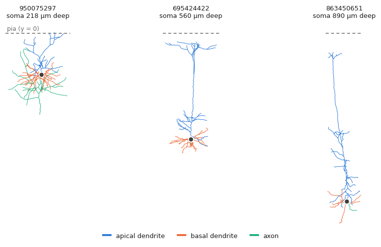
Colour-coded, the three compartments and the reason for separating them are obvious. Note how the apical dendrite (blue) stretches to reach the pia while the basal bush (orange) stays put:
import matplotlib.pyplot as plt

PALETTE = {1: "#3d3d3d", 2: "#1baf7a", 3: "#eb6834", 4: "#2a78d6"}

fig, axes = plt.subplots(1, 3, figsize=(8.2, 4.6))
for ax, n in zip(axes, nl.idx[["ace-nil-mud/950075297_Manual_Upright",
                               "ace-new-let/695424422_Manual_Upright",
                               "ace-net-tug/863450651_Manual_Upright"]]):
    navis.plot2d(n, method="2d", view=("x", "y"), ax=ax,
                 color_by=n.nodes.label.values, palette=PALETTE, lw=0.6)
    ax.axhline(0, color="grey", ls="--", lw=1)  # the pia
Extracting the features#
The call itself is a one-liner:
feats = navis.ivscc_features(nl)
feats.shape
(25, 102)
One row per neuron, 102 columns. Every column is either prefixed with the compartment it describes or is a whole-cell feature:
Prefixed axon_, basal_dendrite_ or apical_dendrite_ and computed on that compartment alone.
| Group | Features |
|---|---|
| Size | num_nodes, total_length, extent_x/y/z |
| Topology | num_branches, num_branch_points, num_tips, max_branch_order |
| Shape | mean_contraction, bifurcation_angle_local, bifurcation_angle_remote |
| Radius | mean_diameter, total_surface, total_volume, parent_daughter_ratio |
| Relative to soma | bias_x, bias_y, soma_percentile_x/y, max_euclidean_distance, max_path_length, early_branch_path |
| Where it leaves | num_stems, exit_distance, exit_theta |
No prefix - these describe the neuron rather than one of its parts.
| Feature | Description |
|---|---|
soma_radius | Radius of the soma node |
soma_surface | Soma surface area, as a sphere |
num_stems | Neurites leaving the soma, across all compartments |
For each ordered pair of compartments, how their depth distributions relate.
| Feature | Description |
|---|---|
<a>_frac_above_<b> | Fraction of a's nodes above b's full depth range |
<a>_frac_intersect_<b> | Fraction of a's nodes inside it |
<a>_frac_below_<b> | Fraction below it |
<a>_emd_with_<b> | Earth mover's distance between the two depth distributions |
The three fractions partition a's nodes and so sum to 1. The EMD is symmetric and therefore recorded once per pair, not twice.
Picking one cell and a handful of columns:
feats.loc["ace-new-let/695424422_Manual_Upright",
          ["apical_dendrite_total_length", "apical_dendrite_num_tips",
           "apical_dendrite_max_branch_order", "apical_dendrite_extent_y",
           "basal_dendrite_total_length", "basal_dendrite_extent_y",
           "num_stems", "soma_radius"]].round(2)
apical_dendrite_total_length         3137.62
apical_dendrite_num_tips               27.00
apical_dendrite_max_branch_order       13.00
apical_dendrite_extent_y              553.22
basal_dendrite_total_length          1890.64
basal_dendrite_extent_y               132.26
num_stems                              11.00
soma_radius                             6.38
Units in, units out
Features are reported in the neuron's own coordinate units and are never rescaled - we loaded these as microns, so lengths are microns, areas µm², angles degrees (except exit_theta, which is radians). Nothing is normalised, so don't mix neurons in different units in one call.
The coordinate frame is not optional#
Before going any further: here is the thing that will silently ruin your results.
y must be cortical depth
A good half of the IVSCC features - bias_y, soma_percentile_y and every overlap feature - are statements about depth, and they read depth off the y axis, with larger y meaning closer to the pia. NAVis cannot check this for you: an unaligned neuron produces exactly the same columns, filled with numbers that mean nothing. Align first, then measure.
This is why we reached for _Upright rather than _Raw earlier. The _Raw files make the point - same cells, same reconstructions, only the frame differs:
raw = navis.NeuronList([])
for bildid in CELLS:
    raw += bil.get_neurons(bil.list_files(bildid, pattern="*_Raw.swc"), units="um")
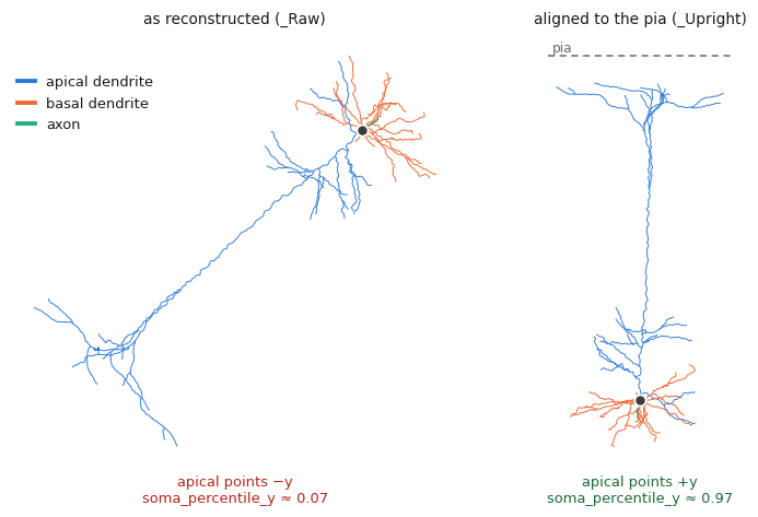
Run those through ivscc_features too, and compare the averages:
feats_raw = navis.ivscc_features(raw)

cols = ["apical_dendrite_soma_percentile_y", "apical_dendrite_bias_y",
        "apical_dendrite_frac_above_basal_dendrite",
        "apical_dendrite_num_tips", "apical_dendrite_num_branch_points"]
pd.DataFrame({"upright": feats[cols].mean(), "raw": feats_raw[cols].mean()}).round(3)
                                           upright      raw
apical_dendrite_soma_percentile_y            0.970    0.066
apical_dendrite_bias_y                     482.040 -421.332
apical_dendrite_frac_above_basal_dendrite    0.694    0.000
apical_dendrite_num_tips                    31.280   31.280
apical_dendrite_num_branch_points           22.120   22.120
In the raw frame the apical dendrite appears to sit below the soma (soma_percentile_y 0.97 0.07) and bias_y flips sign outright - these files use image coordinates, where y grows downwards. Not one of those depth numbers is usable.
The counts, meanwhile, are bit-identical: num_tips and num_branch_points are properties of the tree, not of the frame it is drawn in.
How do I get my own neurons upright?
If your data doesn't ship a pre-aligned variant you have to build the transform yourself - there is no one-size rotation. Two common routes: register to a template brain with navis.xform_brain (see the transforms tutorial), or, if you know two points on the pia and white matter, construct the rotation and apply it with navis.xform. Flipping a sign is enough when the axis is right but points the wrong way:
for n in nl:
    n.nodes["y"] *= -1
Reading the overlap features#
The overlap block is the part that is specific to layered cortex, and it is easiest to understand by looking at where the compartments actually sit. Pooled over all 25 cells, each compartment has its own depth signature - the apical piles up in the top 100 µm (the tuft), the basal hugs the somas around 550 µm:
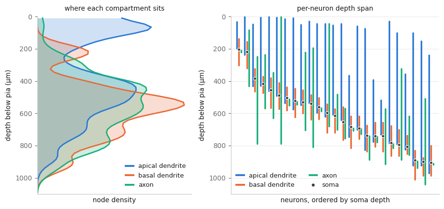
That is exactly what the overlap features put numbers on:
ov = [c for c in feats.columns if "frac_" in c or "emd_" in c]
feats.loc["ace-new-let/695424422_Manual_Upright", ov].round(3)
axon_frac_above_basal_dendrite                     0.000
axon_frac_intersect_basal_dendrite                 1.000
axon_frac_below_basal_dendrite                     0.000
axon_emd_with_basal_dendrite                      12.611
axon_frac_above_apical_dendrite                    0.000
axon_frac_intersect_apical_dendrite                1.000
axon_frac_below_apical_dendrite                    0.000
axon_emd_with_apical_dendrite                    283.479
basal_dendrite_frac_above_axon                     0.376
basal_dendrite_frac_intersect_axon                 0.380
basal_dendrite_frac_below_axon                     0.244
basal_dendrite_frac_above_apical_dendrite          0.000
basal_dendrite_frac_intersect_apical_dendrite      0.865
basal_dendrite_frac_below_apical_dendrite          0.135
basal_dendrite_emd_with_apical_dendrite          279.485
apical_dendrite_frac_above_axon                    0.969
apical_dendrite_frac_intersect_axon                0.014
apical_dendrite_frac_below_axon                    0.017
apical_dendrite_frac_above_basal_dendrite          0.858
apical_dendrite_frac_intersect_basal_dendrite      0.142
apical_dendrite_frac_below_basal_dendrite          0.000
Read the first block as "100% of this axon lies within the depth range spanned by the basal dendrite" - unsurprising, given this cell's axon is a 19-node stub (see the caveats below). The apical dendrite is the informative one: 97% of it sits above the axon and 86% above the basal dendrite. Note that the relationship is not symmetric - only 38% of the basal dendrite sits above the axon, because the two are asking different questions about different reference ranges.
Putting them to work#
A quick demonstration that these features carry real signal. Cortical depth is the organising variable in this dataset, so correlate a few features against it:
# The pia is at y = 0 and cortex runs to negative y, so depth is just -y
soma_depth = pd.Series({n.id: -n.soma_pos[0][1] for n in nl})

for col in ["apical_dendrite_extent_y", "apical_dendrite_bias_y",
            "apical_dendrite_max_path_length", "basal_dendrite_extent_y"]:
    print(f"{col:<34} r = {feats[col].corr(soma_depth):+.2f}")
apical_dendrite_extent_y           r = +0.70
apical_dendrite_bias_y             r = +0.66
apical_dendrite_max_path_length    r = +0.55
basal_dendrite_extent_y            r = +0.06
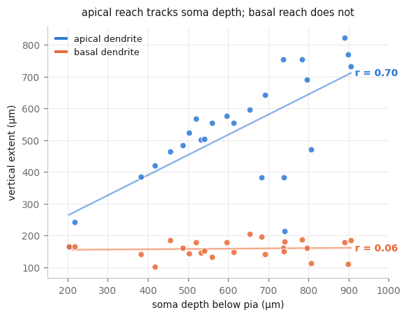
The apical dendrite scales with soma depth - it has further to climb, so it climbs further. The basal dendrite is flat: a compact local bush of much the same size wherever the soma sits. Splitting the compartments is what makes that visible; measured as one tree the two effects would partly cancel.
n = 25
This is a demo, not a result - two dozen cells from mixed Cre lines. Treat the numbers as an illustration of what the features respond to.
Adding your own features#
The feature set is just a list of classes, so you can extend it. Subclass CompartmentFeatures to get a compartment handed to you already subset out, record whatever you like, and pass it via features:
from navis.morpho.ivscc import CompartmentFeatures


class ApicalTuftFeatures(CompartmentFeatures):
    """Fraction of the apical dendrite sitting in the top 200 µm of cortex."""

    compartment = "apical_dendrite"

    def extract_features(self):
        y = self.neuron.nodes.y.values  # `self.neuron` is just the apical dendrite
        self.record_feature("frac_in_tuft", float((y > -200).mean()))
        return self.features


tuft = navis.ivscc_features(nl, features=[ApicalTuftFeatures])
print("correlation with soma depth: %+.2f"
      % tuft.apical_dendrite_frac_in_tuft.corr(soma_depth))
correlation with soma depth: -0.90
What you get inside a feature class
| Attribute | What it is |
|---|---|
self.neuron | the compartment, already subset out (the full neuron for non-compartment classes) |
self.ctx.neuron | the whole neuron, rooted at its soma |
self.ctx.dist_to_root | geodesic distance from every node to the soma, computed once and shared |
self.soma, self.soma_pos, self.soma_radius | soma node ID, position and radius |
self.record_feature(name, value) | records a feature, prefixing it with the compartment name |
Call super().extract_features() first if you want the standard features plus yours, and note that features= replaces the default list - pass DEFAULT_FEATURES + [MyFeatures] to add to it.
Caveats#
Two things worth knowing before you trust a column.
Patch-seq axons are cut off
A slice is 300 µm thick and axons leave it. In this set the axons run from 13 µm to 3.7 mm of cable and 12 of the 25 cells have an axon with no branch point at all - so their axon_bifurcation_angle_* are NaN and their axon_total_length says more about the slice than about the cell. Dendrite features are largely fine; axon features from slice data are not comparable across cells.
Not every cell has every compartment - interneurons have no apical dendrite, and a reconstruction may simply not include the axon. missing_compartments decides what happens then:
| Value | Behavior |
|---|---|
"ignore" (default) | Skip that compartment. Its columns are NaN for that neuron |
"skip" | Drop the neuron from the result entirely |
"raise" | Raise a CompartmentNotFoundError |
The same applies to a neuron with no label column at all - it counts as "no compartments found" rather than an error, so a mixed batch won't blow up on you.
Where next#
- IVSCC on EM data - getting MICrONS reconstructions into a state where these features mean something
- Analyze morphology - the general-purpose morphometrics, for neurons that aren't cortical
- Label propagation and axon-dendrite splits - ways to get compartment labels when your data doesn't come with them
- Cortical neurons - plotting this kind of data, arranged by soma depth
- NBLAST - comparing neurons by shape rather than by feature vector
# *[IVSCC]: In Vitro Single Cell Characterization - the Allen Institute's pipeline for profiling cortical neurons.
# *[SWC]: A plain-text format storing a neuron skeleton as a table of connected nodes.
# *[Patch-seq]: Recording a cell electrophysiologically, then extracting its contents for sequencing and staining it for morphology.
# *[EM]: Electron Microscopy.
# *[EMD]: Earth mover's distance - the cost of turning one distribution into another.
# *[BIL]: Brain Image Library.
Total running time of the script: ( 0 minutes 0.000 seconds)
Download Python source code: zzz_tutorial_morpho_05_ivscc.py
Download Jupyter notebook: zzz_tutorial_morpho_05_ivscc.ipynb