Note
Click here to download the full example code
Skeletons#
Fine-tune skeleton figures: radii, tapering, halos and depth sorting.
Skeletons are lines, and lines are what matplotlib is best at - so plot2d gives you considerably more control here than any of the 3D backends. If you have not read the plotting overview yet, start there; for colors and palettes see coloring, which works the same in every backend.
| Parameter | Effect | Works in plot3d? |
|---|---|---|
radius | Draw skeletons as tubes (True/"auto"/"lw") or lines (False) | |
linewidth | Line thickness - also scales the tubes when radius=True; default 1 | |
linestyle | Dash style, e.g. "--" (only when radius=False); default "-" | |
taper | Width from "strahler" or "subtree" instead of a constant | |
halo | Background-coloured outline, so crossings read as one neuron in front | |
depth_sort | Interleave neurons by depth instead of drawing them one after another | |
style | A named bundle of the above, e.g. "publication" |
All of these need method="2d" unless the table says otherwise.
Radii#
If your skeletons have radii - a non-empty radius column in their .nodes table - you can draw them as tubes rather than lines. The default is False, because tubes are slower for big scenes.
import navis
import matplotlib.pyplot as plt

n = navis.example_neurons(1, kind="skeleton")

fig, axes = plt.subplots(1, 4, figsize=(16, 5))
for ax, (title, kwargs) in zip(
    axes,
    [
        ("radius=False (default)", dict(radius=False)),
        ("radius=True", dict(radius=True)),
        ("radius=True, linewidth=2", dict(radius=True, linewidth=2)),
        ('radius="lw"', dict(radius="lw")),
    ],
):
    navis.plot2d(n, ax=ax, method="2d", view=("x", "-z"), **kwargs)
    ax.set_title(title, fontsize=11, y=0.98)
    ax.set_axis_off()
plt.tight_layout()
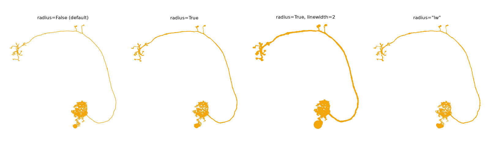
The four modes:
| Value | What you get |
|---|---|
False | Plain lines at linewidth points |
True | Tubes outlined in the view plane, scaled by linewidth |
"auto" | Tubes if the neuron has usable radii, lines otherwise - the safe choice for a NeuronList |
"lw" | Radius mapped onto the line width instead of an outline |
When to use radius=\"lw\"
It looks near-identical to radius=True, gets exact round joins for free and more than halves the size of vector output. The catch: line widths are in points, so the data-to-points conversion is redone on every draw - which makes it a little slower to render, and only correct on axes it can measure.
Line width and style#
linewidth (alias lw) is the thickness in points, and doubles as the scaling factor for radius. linestyle (alias ls) takes any matplotlib dash pattern - but only where the neurites are actually lines, so it does nothing under radius=True:
fig, axes = plt.subplots(1, 3, figsize=(13, 5))
for ax, (title, kwargs) in zip(
    axes,
    [
        ("linewidth=1", dict(linewidth=1)),
        ("linewidth=2", dict(linewidth=2)),
        ('linewidth=2, linestyle="--"', dict(linewidth=2, linestyle="--")),
    ],
):
    navis.plot2d(n, ax=ax, method="2d", view=("x", "-z"), **kwargs)
    ax.set_title(title, fontsize=11, y=0.98)
    ax.set_axis_off()
plt.tight_layout()
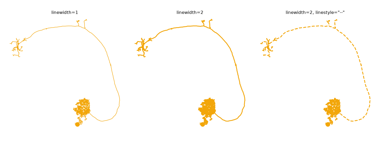
linestyle is matplotlib-only
radius and linewidth also work with plot3d; linestyle does not.
Tapering without radii#
Radii are often missing or a placeholder. You can still taper a skeleton using its topology, which gets you most of the way to the look of a real morphology. "strahler" follows the Strahler index - chunky and categorical, so it shows the branch hierarchy - while "subtree" follows how much cable hangs below each node, which is smooth:
fig, axes = plt.subplots(1, 3, figsize=(13, 5))
for ax, taper in zip(axes, [None, "strahler", "subtree"]):
    navis.plot2d(n, ax=ax, method="2d", view=("x", "-z"), taper=taper)
    ax.set_title(f"taper={taper!r}", fontsize=11, y=0.98)
    ax.set_axis_off()
plt.tight_layout()
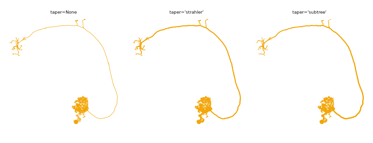
Widths run from 0.35x to 3.5x linewidth, so linewidth still scales the whole thing. taper is ignored when the neurites are drawn with radius.
Halos#
In a scene with more than a handful of neurons, the pile of crossings is what makes a plot unreadable. A halo draws each neuron with an outline in the background colour underneath it, so a crossing reads as one neuron passing in front of another:
nl = navis.example_neurons(5, kind="skeleton")

fig, axes = plt.subplots(1, 3, figsize=(15, 5.5))
for ax, kwargs in zip(
    axes, [dict(halo=False), dict(halo=3), dict(halo=3, depth_sort=True)]
):
    navis.plot2d(nl, ax=ax, method="2d", view=("x", "-z"), linewidth=1.5, **kwargs)
    ax.set_title(", ".join(f"{k}={v!r}" for k, v in kwargs.items()), fontsize=11, y=0.98)
    ax.set_axis_off()
plt.tight_layout()
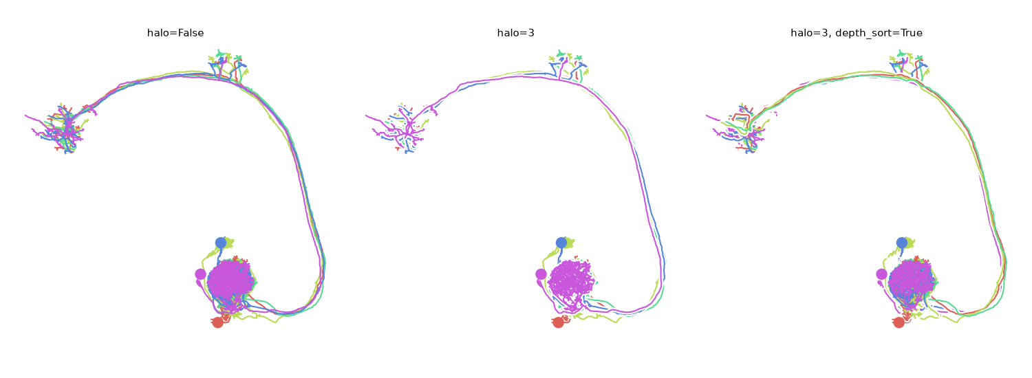
halo=True uses 3 points; a number sets the width. The colour comes from the axes background, which is usually what you want - on a dark background pass it explicitly as halo={"width": 4, "color": "k"}.
The halo marks whichever neuron is in front, so it is only as good as the ordering underneath it. On its own (middle panel) "in front" just means "later in the input", and the last neuron cuts a clean channel through all the others. Add depth_sort (right panel) and the crossings start resolving the way the anatomy actually does - which is why the two usually travel together.
Depth sorting#
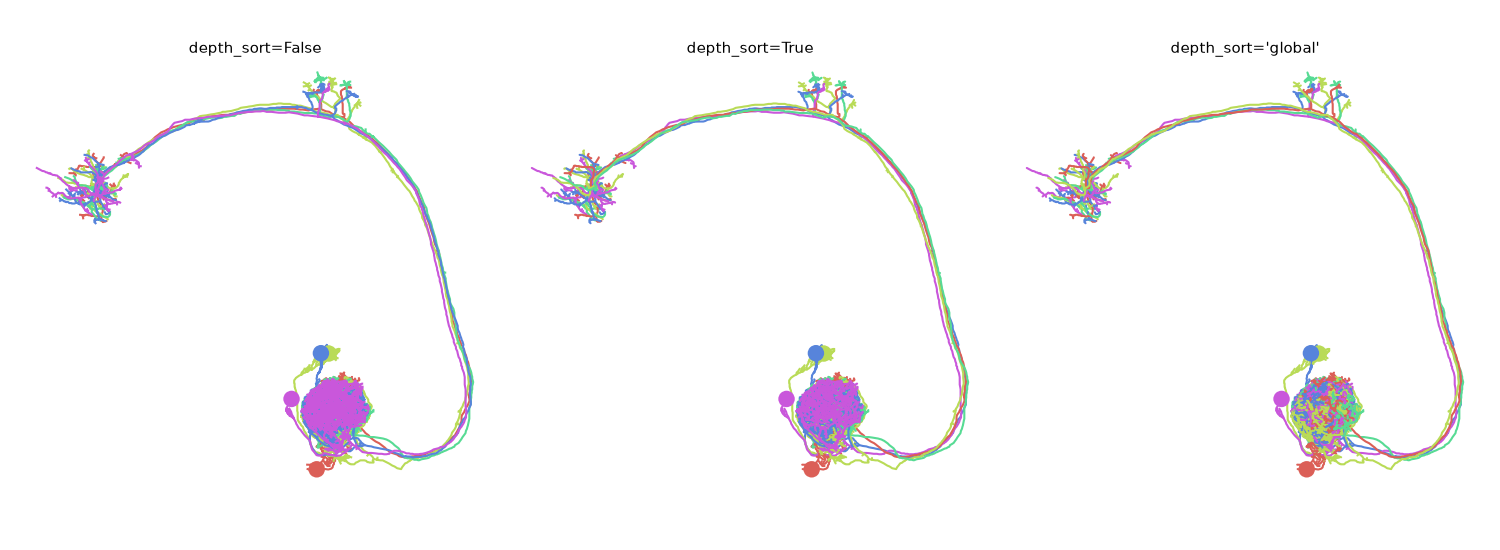
By default neurons are drawn one after another, so the last one is always on top no matter where it sits in Z. depth_sort puts them into one stack instead - as close to real occlusion as matplotlib gets. It comes in two flavours:
| Value | How | Cost |
|---|---|---|
True/int | Bucket everything into N bins along the depth axis (True = 10) | One artist per bin per neuron |
"global" | Sort exactly, merging each neuron type into one artist | Cheaper than 10 bins, for skeletons |
fig, axes = plt.subplots(1, 3, figsize=(15, 5.5))
for ax, ds in zip(axes, [False, True, "global"]):
    navis.plot2d(nl, ax=ax, method="2d", view=("x", "-z"), linewidth=1.5, depth_sort=ds)
    ax.set_title(f"depth_sort={ds!r}", fontsize=11, y=0.98)
    ax.set_axis_off()
plt.tight_layout()
Bins cost artists
Each bin is one artist per neuron (two with halo), so hundreds of neurons at 10 bins means thousands of artists. Lower the bin count for big scenes - or use "global", which is one artist however many neurons you have.
Pass a negative number (e.g. depth_sort=-10) to flip which end of the depth axis counts as nearest the viewer. "global" always follows the view.
"global" and halo do not mix
A halo has to sit between two neurons, and a single merged artist has nowhere to put it. Passing both warns and falls back to bins. Meshes also pay far more for "global" than skeletons do - see meshes.
Styles#
Rather than remembering which combination you liked, style bundles them under a name:
fig, axes = plt.subplots(1, 2, figsize=(11, 5.5))
for ax, style in zip(axes, [None, "publication"]):
    navis.plot2d(n, ax=ax, method="2d", view=("x", "-z"), style=style)
    ax.set_title(f"style={style!r}", fontsize=11, y=0.98)
    ax.set_axis_off()
plt.tight_layout()
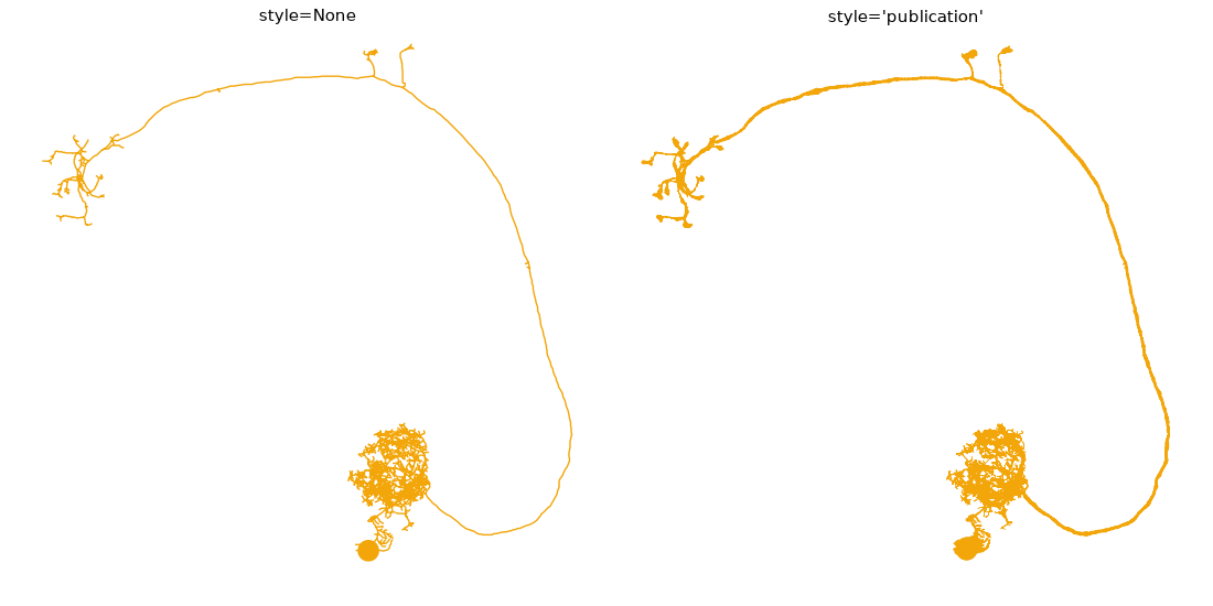
"publication" sets radius="auto", depth_sort=True, soma=True and mesh_shade=True. A style only fills in arguments you did not pass yourself, so you can always override part of it:
navis.plot2d(n, style="publication", radius=False, taper="subtree")
See navis.plotting.dd.PLOT_STYLES for what each style sets.
Plotting meshes or volumes?
Shading, outlines and depth sorting work a little differently for Meshes and Volumes - see meshes and volumes.
Total running time of the script: ( 0 minutes 2.461 seconds)
Download Python source code: tutorial_plotting_2d_00_skeletons.py
Download Jupyter notebook: tutorial_plotting_2d_00_skeletons.ipynb