Volumes#

Put a neuropil around your neurons without losing sight of them.

A Volume in 3D has exactly one hard problem: it is a closed shell, and you want to see what is inside it. Everything below is about that trade-off - and about the fact that a real renderer, unlike plot2d, composites the shell correctly whichever way you turn it.

If you have not read the plotting overview yet, start there. The 2D counterpart to this page is 2D volumes.

Parameter	Effect	octarine	plotly	k3d
`color`/`alpha`	Volumes carry a default colour and alpha of their own
`lighting`	Lighting preset - `"rim"` is made for translucent shells
`volume_legend`	Give volumes their own legend entries
`snapshot`	Render offscreen into a `matplotlib` figure

The interactive viewer#

A neuropil goes into the scene like anything else. Interactively it is also the easiest way to handle the shell problem - rotate until the neuron clears it, rather than agonising over an alpha:

import navis
import matplotlib.pyplot as plt

n = navis.example_neurons(1, kind="skeleton")
lh = navis.example_volume("LH")

navis.plot3d([n, lh], backend="plotly", lighting="rim", legend=False, height=600)

Lighting a shell (plotly)#

That is the "rim" preset, and it exists for exactly this case: a bright Fresnel edge gives the shell enough form to read as a solid without filling in the middle, so whatever is inside stays visible.

Preset	On a translucent neuropil
`"default"`	Dimensional, even shading across the shell
`"matte"`	Softest - the least distracting behind a busy scene
`"rim"`	Bright at grazing angles, near-clear face-on
`False`	Plotly's flat default - the shell reads as a solid colour

Legends

volume_legend=True gives volumes their own legend entries so viewers can click them on and off - which is often better than picking an alpha at all:

navis.plot3d([n, lh], backend="plotly", volume_legend=True)

Alpha is the whole game#

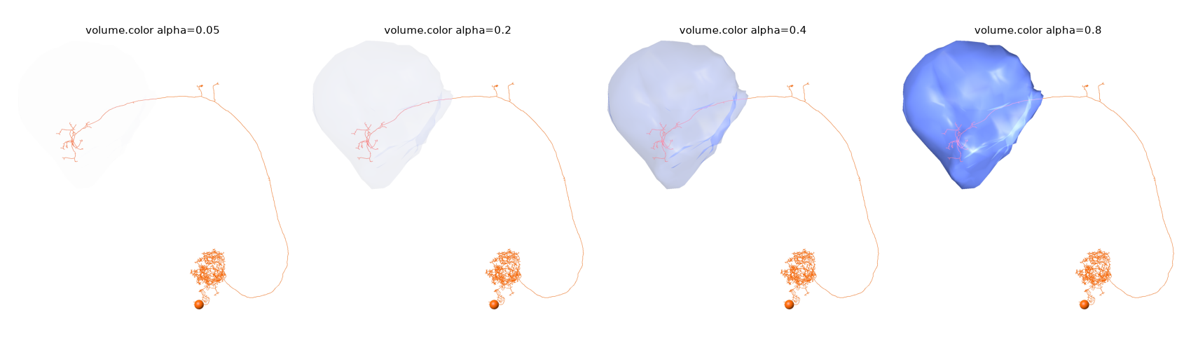
For a static figure you do have to pick an alpha. Volumes default to a pale grey at 20% opacity, which is usually about right. Push it up and the neuron disappears; push it down and the neuropil stops reading as a shape. Here rendered with snapshot=True, which puts the octarine render onto a matplotlib axes so the settings can sit side by side:

fig, axes = plt.subplots(1, 4, figsize=(17, 5))
for ax, alpha in zip(axes, [0.05, 0.2, 0.4, 0.8]):
    lh.color = (0.4, 0.5, 0.9, alpha)
    navis.plot3d([n, lh], snapshot=True, ax=ax, view=("x", "-z"), color="#F76707")
    ax.set_title(f"volume.color alpha={alpha}", fontsize=11, y=0.98)
    ax.set_axis_off()
plt.tight_layout()

Colour volumes via .color, not color=

With the octarine backend a volume takes its colour from its own .color attribute; the color= argument only reaches neurons. The plotly and k3d backends do honour color={volume.name: ...}, as does plot2d - so setting .color on the volume is the one approach that works everywhere.

Look at the last two panels: the shell darkens where the surface folds over itself, because you are seeing through two layers of it. That is correct, and it is the sort of thing a real renderer gets right for free. In 2D, NAVis has to fill the union of the visible faces as a single path to stop the same effect turning into an artefact.

Several volumes#

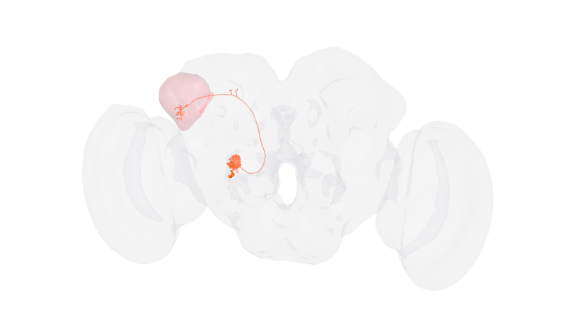
A big outer shell at low alpha and a small inner one at higher alpha is the standard recipe: the brain outline says where, the neuropil says which, and the neuron stays legible through both.

brain = navis.example_volume("neuropil")

lh.color = (0.9, 0.3, 0.3, 0.35)
brain.color = (0.5, 0.5, 0.6, 0.18)

# no `figsize`: the figure then matches the render's own aspect ratio, and a brain is much
# wider than it is tall
navis.plot3d([n, lh, brain], snapshot=True, view=("x", "-z"), color="#F76707")

Out:

(<Figure size 806.723x480 with 1 Axes>, <Axes: >)

Low alpha plus a big mesh is a trap

Two things happen when you add a whole-brain outline. It rescales the scene - the camera now has to fit the entire brain, so the neuron shrinks to a fraction of the frame - and a shell that large is spread very thin, so an alpha that looked fine on a small neuropil can vanish altogether. Below ~0.1 the brain above is effectively invisible while still costing you all that framing. If a volume seems to have disappeared but the plot got bigger, this is why: raise the alpha, or drop the outer shell and let the inner one do the work.

Cameras and cutaways#

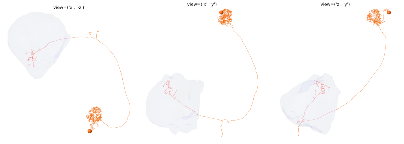
There is no clipping plane, but a well-chosen camera does much of the same work. Since view accepts a camera state dict, the usual workflow is to find the angle interactively and then render it:

viewer = navis.plot3d([n, lh])   # spin until the neuropil is edge-on
state = viewer.get_view()
navis.plot3d([n, lh], snapshot=True, view=state, figsize=(7, 7))

Axis-aligned views often suffice:

lh.color = (0.4, 0.5, 0.9, 0.18)

fig, axes = plt.subplots(1, 3, figsize=(14, 5))
for ax, view in zip(axes, [("x", "-z"), ("x", "y"), ("z", "y")]):
    navis.plot3d([n, lh], snapshot=True, ax=ax, view=view, color="#F76707")
    ax.set_title(f"view={view}", fontsize=11, y=0.98)
    ax.set_axis_off()
plt.tight_layout()

2D or 3D for a figure with context?#

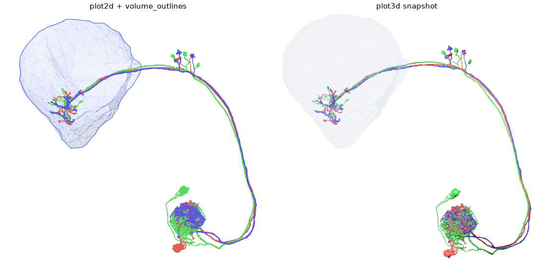
Both are defensible, and it comes down to what you need out of the file:

nl = navis.example_neurons(3, kind="skeleton")

fig, axes = plt.subplots(1, 2, figsize=(11, 5.5))
navis.plot2d(
    [nl, lh], ax=axes[0], method="2d", view=("x", "-z"),
    style="publication", volume_outlines="both",
)
axes[0].set_title("plot2d + volume_outlines", fontsize=11, y=0.98)
navis.plot3d([nl, lh], snapshot=True, ax=axes[1], view=("x", "-z"), radius=True)
axes[1].set_title("plot3d snapshot", fontsize=11, y=0.98)
for ax in axes:
    ax.set_axis_off()
plt.tight_layout()

	`plot2d`	`plot3d` with `snapshot`
Output	Vector - editable, scales forever	Raster
Occlusion	Approximated (`depth_sort`, culling)	Real
Neuropil	A contour, which is often cleaner in print	A lit shell
Camera	Axis-aligned views only	Anything

A common compromise: render the 3D scene to a snapshot and then annotate it in matplotlib, since the image sits in data coordinates - see 3D skeletons for a scale bar built that way.

Total running time of the script: ( 0 minutes 6.509 seconds)

Download Python source code: tutorial_plotting_3d_02_volumes.py

Download Jupyter notebook: tutorial_plotting_3d_02_volumes.ipynb

Gallery generated by mkdocs-gallery