Note
Click here to download the full example code
Meshes#
Shade, outline and stack mesh neurons.
The mesh counterpart to the skeleton tutorial. If you have not read the plotting overview yet, start there; for colors and palettes see coloring.
As with skeletons we focus on plot2d with method="2d": matplotlib gives us a flat canvas we can project onto ourselves, which turns out to be both faster and better looking than handing the geometry to matplotlib's own 3D machinery.
| Parameter | Effect | Works in plot3d? |
|---|---|---|
mesh_shade | Light the surface: True, "cel", "rim" or "ghost" | |
alpha | Opacity - correct now even where the surface folds over itself | |
color_by | Per-vertex colours; shading multiplies into them rather than replacing | |
halo | Background-coloured outline, so crossings read as one neuron in front | |
depth_sort | Bin mesh faces with the skeletons, or "global" to sort them exactly | |
style | A named bundle of the above, e.g. "publication" |
Neuropils are meshes too, but they behave differently enough to get their own tutorial.
Occlusion comes for free#
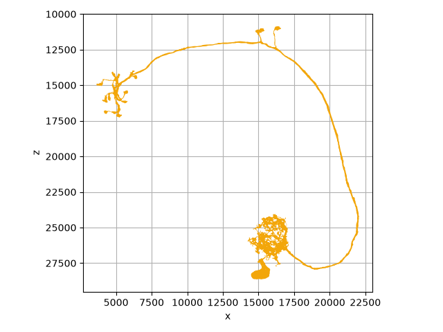
There is nothing to switch on here - it is worth knowing about because it changed. Faces pointing away from the viewer are dropped and the rest painted furthest-first, so a mesh now has a front and a back. Before, faces went down in whatever order the mesh happened to store them.
Culling roughly halves the polygons that reach the renderer, so this is also faster than what it replaced.
import navis
import matplotlib.pyplot as plt

m = navis.example_neurons(1, kind="mesh")

fig, ax = navis.plot2d(m, view=("x", "-z"), method="2d")
plt.tight_layout()
Shading#
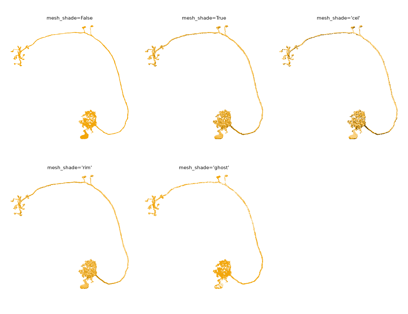
mesh_shade lights the surface. At whole-cell zoom a neurite is only a pixel or two wide, so this mostly shows on the soma and the thick primary neurite - zoom into an arbour and it does a lot more:
fig, axes = plt.subplots(2, 3, figsize=(13, 10))
for ax, shade in zip(axes.flat, [False, True, "cel", "rim", "ghost"]):
    navis.plot2d(m, ax=ax, method="2d", view=("x", "-z"), mesh_shade=shade)
    ax.set_title(f"mesh_shade={shade!r}", fontsize=11, y=0.98)
for ax in axes.flat:
    ax.set_axis_off()  # also blanks the unused sixth panel
plt.tight_layout()
| Mode | What it does |
|---|---|
True | Plain diffuse (Lambertian) shading. The one to reach for |
"cel" | The same, posterised into three tones - diagrammatic, and the smallest vector output |
"rim" | Diffuse plus a bright rim at grazing angles, which separates touching tubes |
"ghost" | Opacity from the grazing angle instead of brightness - see volumes |
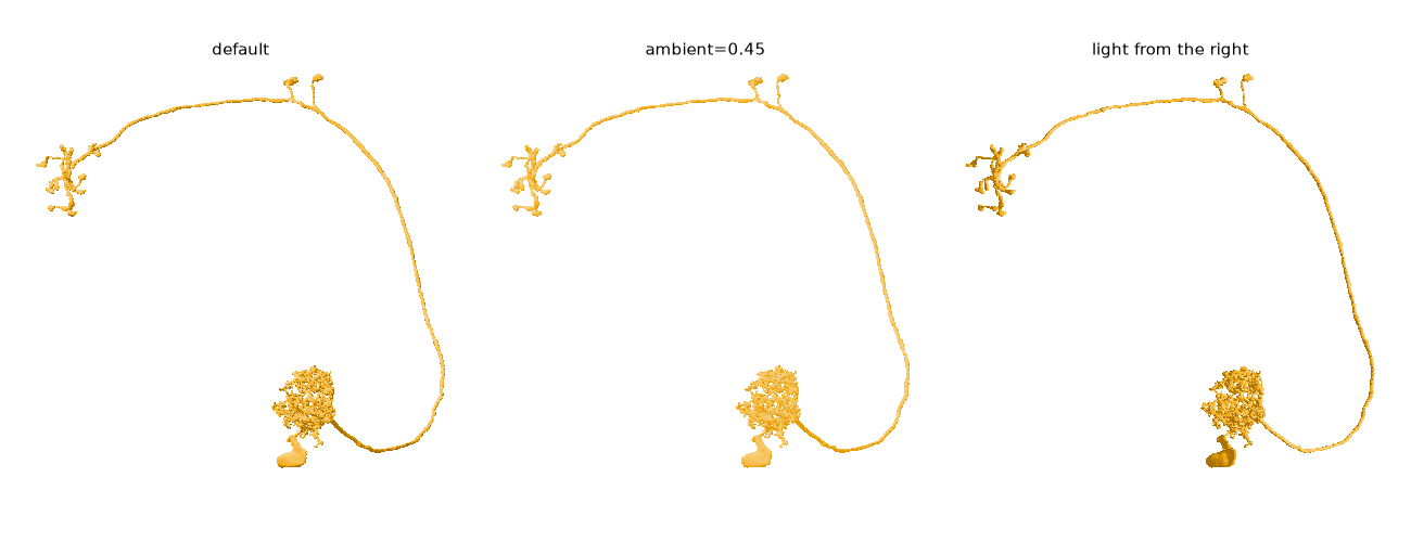
Pass a dict to tune it. light is a direction in view space (x right, y up, z towards you), so it follows the camera rather than the data; ambient sets how much light a face gets when it points straight away from the key light:
fig, axes = plt.subplots(1, 3, figsize=(13, 5))
for ax, (title, shade) in zip(
    axes,
    [
        ("default", True),
        ("ambient=0.45", {"mode": "lambert", "ambient": 0.45}),
        ("light from the right", {"mode": "lambert", "light": (1, 0.2, 0.6)}),
    ],
):
    navis.plot2d(m, ax=ax, method="2d", view=("x", "-z"), mesh_shade=shade)
    ax.set_title(title, fontsize=11, y=0.98)
    ax.set_axis_off()
plt.tight_layout()
mesh_shade in 3D
plot3d and method="3d" understand mesh_shade as a plain on/off switch - the mode names are specific to method="2d", which is where we do the projection ourselves. For real lighting controls see 3D meshes.
Shading and colours#
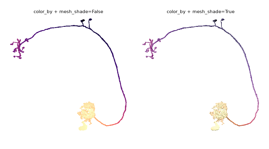
Shading multiplies into whatever colour a face already has instead of replacing it, so it composes with everything else - color, color_by and depth_coloring alike:
fig, axes = plt.subplots(1, 2, figsize=(9, 5))
for ax, shade in zip(axes, [False, True]):
    navis.plot2d(
        m,
        ax=ax,
        method="2d",
        view=("x", "-z"),
        color_by=m.vertices[:, 1],  # colour by depth into the screen
        palette="magma",
        mesh_shade=shade,
    )
    ax.set_title(f"color_by + mesh_shade={shade}", fontsize=11, y=0.98)
    ax.set_axis_off()
plt.tight_layout()
Transparency#
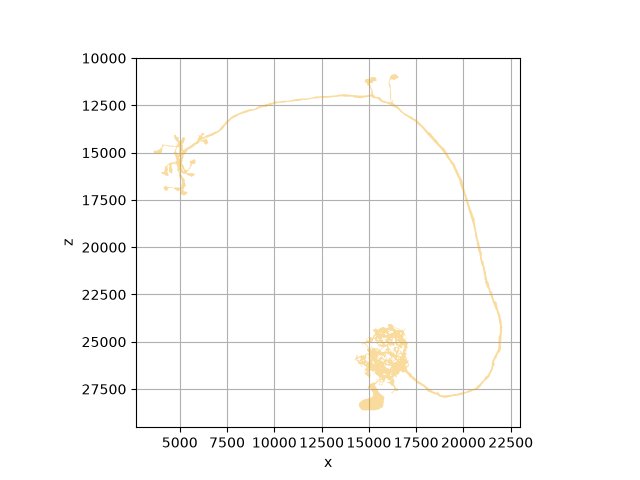
A mesh in one colour is filled as a single path, which means alpha finally means what it says. Previously every triangle was composited on its own, so a fold in the surface came out darker than a flat stretch and the neuron looked solid where it was merely doubled over:
fig, ax = navis.plot2d(m, view=("x", "-z"), method="2d", alpha=0.4)
Shading gives that up again
Shading needs a colour per face, which rules out the single-path fill. Where a translucent mesh overlaps itself the shaded version double-darkens instead of filling once. If that matters more to you than the lighting does, pass mesh_shade=False.
Halos#
Meshes take the same halo as skeletons: an outline in the background colour, drawn underneath, so a crossing reads as one neuron passing in front of another.
nl = navis.example_neurons(3, kind="mesh")

fig, axes = plt.subplots(1, 3, figsize=(15, 5.5))
for ax, kwargs in zip(
    axes, [dict(halo=False), dict(halo=3), dict(halo=3, depth_sort=True)]
):
    navis.plot2d(nl, ax=ax, method="2d", view=("x", "-z"), **kwargs)
    ax.set_title(", ".join(f"{k}={v!r}" for k, v in kwargs.items()), fontsize=11, y=0.98)
    ax.set_axis_off()
plt.tight_layout()
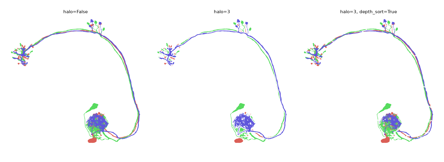
As with skeletons, the halo only marks what is already in front: without depth_sort that is simply the last mesh in the input, so the third neuron carves a channel through the other two.
The right panel is where meshes part company with skeletons. Binning slices each mesh's outline into depth layers, and every layer strokes its own halo - so a neurite that crosses a bin boundary gets nicked by its own halo, and the primary neurite comes out looking dashed. For meshes, halo alone or depth_sort alone usually reads better than the two together; if you do need both, fewer bins means fewer seams.
Halos are slow on dense arbours
The outline is the neuron's own path stroked underneath its fill, and that path has one subpath per visible triangle. It rasterises slowly. Pair it with rasterize=True for big scenes.
Keylines instead of halos
The halo is drawn by stroking the mesh's own outline underneath its fill, so passing a thin dark colour instead of the background gives you an ink-on-paper keyline:
navis.plot2d(m, halo={"width": 1, "color": "#2a3f7a"}, mesh_shade=True)
Depth sorting#
By default a mesh is one artist drawn over the skeletons, whatever its actual depth. depth_sort puts its faces into the same stack skeleton nodes go into - either binned, or sorted exactly:
fig, axes = plt.subplots(1, 3, figsize=(15, 5.5))
for ax, ds in zip(axes, [False, 20, "global"]):
    navis.plot2d(nl, ax=ax, method="2d", view=("x", "-z"), depth_sort=ds)
    ax.set_title(f"depth_sort={ds!r}", fontsize=11, y=0.98)
    ax.set_axis_off()
plt.tight_layout()
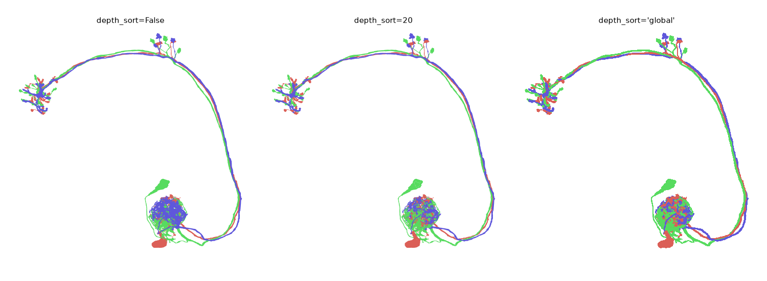
The difference shows where neurons pile up - in the glomerulus above, depth_sort is what stops the last neuron drawn from owning the whole thing. Bins are an approximation: faces in the same bin still fall back to draw order, whereas "global" merges every mesh into one artist and sorts all their faces together, so two neurons interleave face by face.
"global" is the expensive mode for meshes
A flat mesh is normally a single filled outline, and sorting across neurons forces it down to one polygon per face - on the example neurons that is several times the cost of either the default or the bins, and it gives up the fill-once alpha along with it. It is a finished-figure setting, not an exploration one. Skeletons get off far more lightly; see the skeleton tutorial.
All of the above at once#
style="publication" bundles the settings you would otherwise reach for one by one - for meshes that is mesh_shade and depth_sort (plus radius and soma, which only skeletons care about):
fig, axes = plt.subplots(1, 2, figsize=(11, 5.5))
for ax, style in zip(axes, [None, "publication"]):
    navis.plot2d(nl, ax=ax, method="2d", view=("x", "-z"), style=style)
    ax.set_title(f"style={style!r}", fontsize=11, y=0.98)
    ax.set_axis_off()
plt.tight_layout()
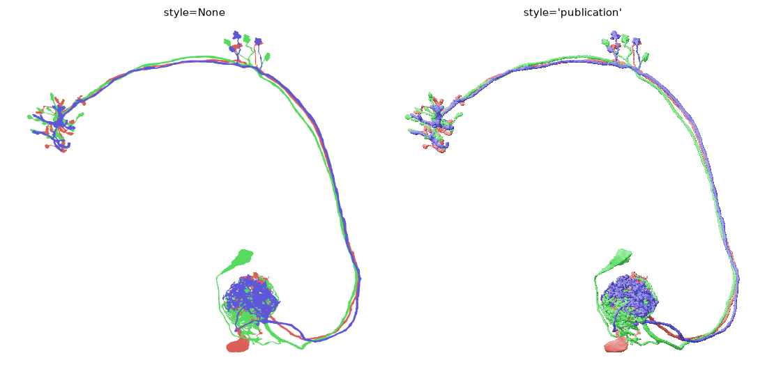
A style only fills in what you did not pass yourself, so you can still opt out of any part of it - style="publication", mesh_shade=False gets you the depth sorting and a flat fill.
Total running time of the script: ( 0 minutes 5.465 seconds)
Download Python source code: tutorial_plotting_2d_01_meshes.py
Download Jupyter notebook: tutorial_plotting_2d_01_meshes.ipynb