Note

Click here to download the full example code

Skeletons from light-level data

Extract skeletons from confocal microscopy image stacks.

This example is not executed

In contrast to almost all other tutorials, this one is not executed when the documentation is built. Consequently, it also does not display any actual code output or plots - images shown are statically embedded. The main reason for this is that the example requires downloading a large-ish file which is a pain in the neck to get to work in the CI environment.

Extracting neuron skeletons from microscopy data is a common but non-trivial task. There are about as many ways to do this as there are people doing it - from fully manual to fully automated tracing.

This tutorial walks through a fully automated pipeline built from a few easy-to-install Python packages. If it isn't for you, check out the Alternatives at the end.

graph LR
    A[Download<br>H5J stack] -->|"Fiji"| B[NRRD file];
    B -->|"nrrd.read()"| C[Threshold];
    C -->|"cc3d"| D[Label<br>components];
    D -->|"kimimaro"| E[Skeletons];
    E -->|"read_swc()"| F[NAVis neurons];

Requirements

This tutorial needs three extra packages - install them all in one go:

pip install pynrrd connected-components-3d kimimaro -U

• pynrrd - load NRRD image stacks
• connected-components-3d (cc3d) - label connected components
• kimimaro - extract the skeletons

Preparing the data

This pipeline was designed for pre-segmented data and does little to handle noise. Fortunately, the image stack we'll use is exceptionally clean, which keeps skeletonization straightforward.

In practice you may need to pre-process your data first. If ordinary thresholding and denoising don't cut it, reach for more advanced segmentation tools such as Ilastik (see its pixel classification and voxel segmentation tutorials) or DeepImageJ.

Download Image Stack

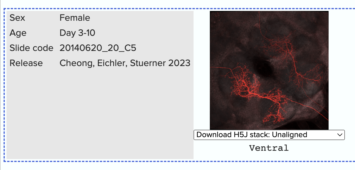
As example data, we will use a confocal stack from the Janelia Split-Gal4 collection. We picked the SS00731 line because it's already fairly clean as is and there are high-resolution stacks with stochastic multi-color labeling of individual neurons available for download.

Scroll all the way to the bottom of the page and in the dropdown for the left-most image, select "Download H5J stack: Unaligned".

Convert to NRRD

H5J isn't a format we can load directly in Python, so we first convert it to NRRD using Fiji/ImageJ.

Converting H5J to NRRD in Fiji

1. Fire up Fiji/ImageJ.
2. Drag & drop the SS00731-...-unaligned_stack.h5j file into Fiji.
3. "Image" → "Colors" → "Split Channels" to split the image into its channels.
4. Discard all but the red "C1" channel (our neurons).
5. "Image" → "Type" → "8-bit" to convert to 8-bit (optional but recommended).
6. "File" → "Save As" → "NRRD" and save as neuron.nrrd.

Extracting the Skeleton

Now that we have that file in a format we can load it into Python, we can get started:

import kimimaro
import nrrd
import navis
import cc3d
import numpy as np

First load the image stack:

# `im` is numpy array, `header` is a dictionary
im, header = nrrd.read(
    "neuron.nrrd"
)

Next we pick a threshold to binarize the image. This isn't strictly necessary, but it's the more intuitive place to start.

# Threshold the image
mask = (im >= 20).astype(np.uint8)

You can inspect the mask to see if the thresholding worked as expected:

import matplotlib.pyplot as plt
plt.imshow(mask.max(axis=2))

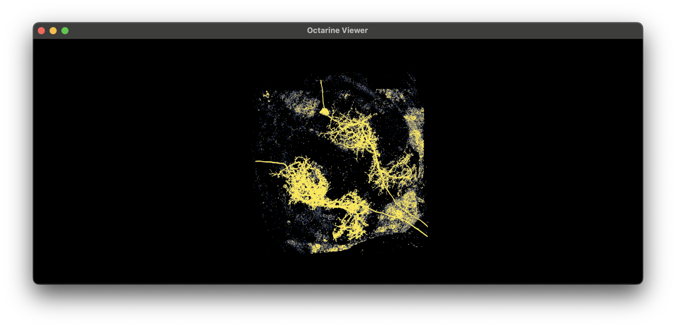
With the octarine backend, you can also visualize the volume in 3D:

# spacing can be found in the `header` dictionary
import octarine as oc
v = oc.Viewer()
v.add_volume(mask, spacing=(.19, .19, .38))

Getting the threshold right

• Test candidate thresholds interactively in e.g. ImageJ/Fiji.
• Remove as much background as possible without disconnecting neurites.
• Perfection is the enemy of progress - we can denoise and reconnect during post-processing.

Next, label the connected components in the image:

Extract the labels

labels, N = cc3d.connected_components(mask, return_N=True)

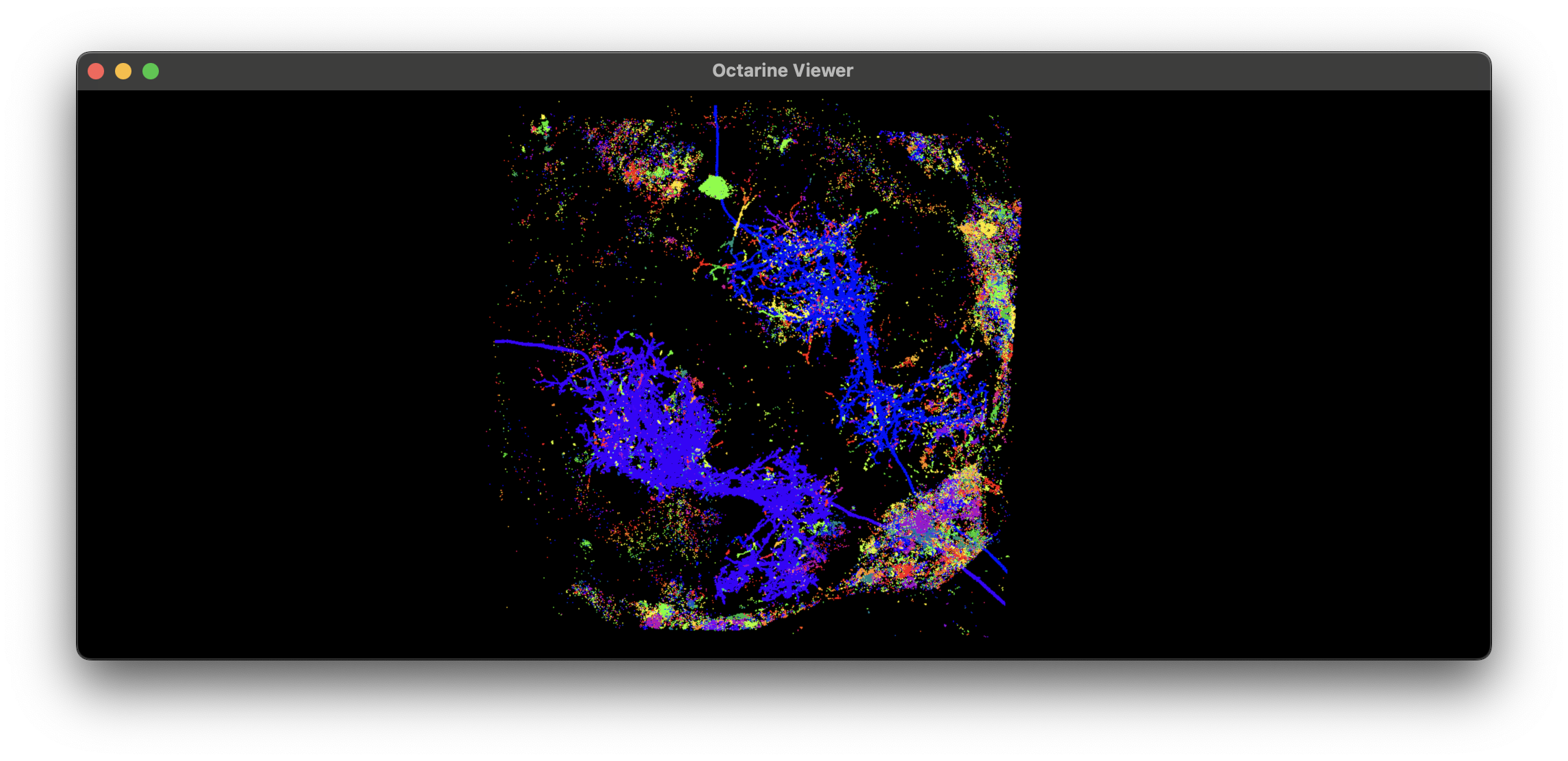
Visualize the labels:

import cmap
import octarine as oc
v = oc.Viewer()
v.add_volume(labels, spacing=(.19, .19, .38), color=cmap.Colormap('prism'))

Experiment

cc3d.connected_component also works with non-thresholded image - see the delta parameter.

# Collect some statistics
stats = cc3d.statistics(labels)

print("Total no. of labeled components:", N)
print("Per-label voxel counts:", np.sort(stats["voxel_counts"])[::-1])
print("Label IDs:", np.argsort(stats["voxel_counts"])[::-1])

Total no. of labeled components: 37836
Per-label voxel counts: [491996140    527374    207632 ...         1         1         1]
Label IDs: [    0  6423  6091 ... 22350 22351 18918]

Note how label 0 has suspiciously many voxels? That's because this is the background label. We need to make sure to exclude it from the skeletonization process:

to_skeletonize = np.arange(1, N)

Now run the actual skeletonization.

Skeletonization parameters

A handful of parameters are worth tweaking for your data - the key ones are called out in the annotations below. See the kimimaro repository for the full list and a detailed explanation.

skels = kimimaro.skeletonize(
    labels,
    teasar_params={
        "scale": 1.5,                      # (1)!
        "const": 1,                        # physical units (1 micron in our case)
        "pdrf_scale": 100000,
        "pdrf_exponent": 4,
        "soma_acceptance_threshold": 3.5,  # physical units
        "soma_detection_threshold": 1,     # physical units
        "soma_invalidation_const": 0.5,    # physical units
        "soma_invalidation_scale": 2,
        "max_paths": None,                 # (2)!
    },
    object_ids=list(to_skeletonize),       # (3)!
    dust_threshold=500,                    # (4)!
    anisotropy=(0.19, .19, 0.38),          # (5)!
    progress=True,                         # show progress bar
    parallel=6,                            # (6)!
    parallel_chunk_size=1,                 # skeletons processed before updating the progress bar
)

1. Together with const, controls skeleton detail: lower values = more detail but more noise.
2. Cap on paths processed per skeleton. Set it low to finish early, e.g. for a quick test (None = no cap).
3. Only process these labels - remember we dropped the background label 0.
4. Skip connected components with fewer than this many voxels.
5. Voxel size in physical units - check the header dict for your image's spacing.
6. Parallelism: <= 0 uses all CPUs, 1 runs single-process, 2+ uses multiprocessing.

skels is a dictionary of {label: cloudvolume.Skeleton}. Let's convert these to NAVis neurons:

# Convert skeletons to NAVis neurons
nl = navis.NeuronList([navis.read_swc(s.to_swc(), id=i) for i, s in skels.items()])

Based on the voxel sizes in stats, we can make an educated guess that label 6423 is one of our neurons. Let's visualize it in 3D:

import octarine as oc
v = oc.Viewer()
v.add_neurons(nl.idx[6423], color='r', linewidth=2, radius=False))
v.add_volume(im, spacing=(.19, .19, .38), opacity=.5)

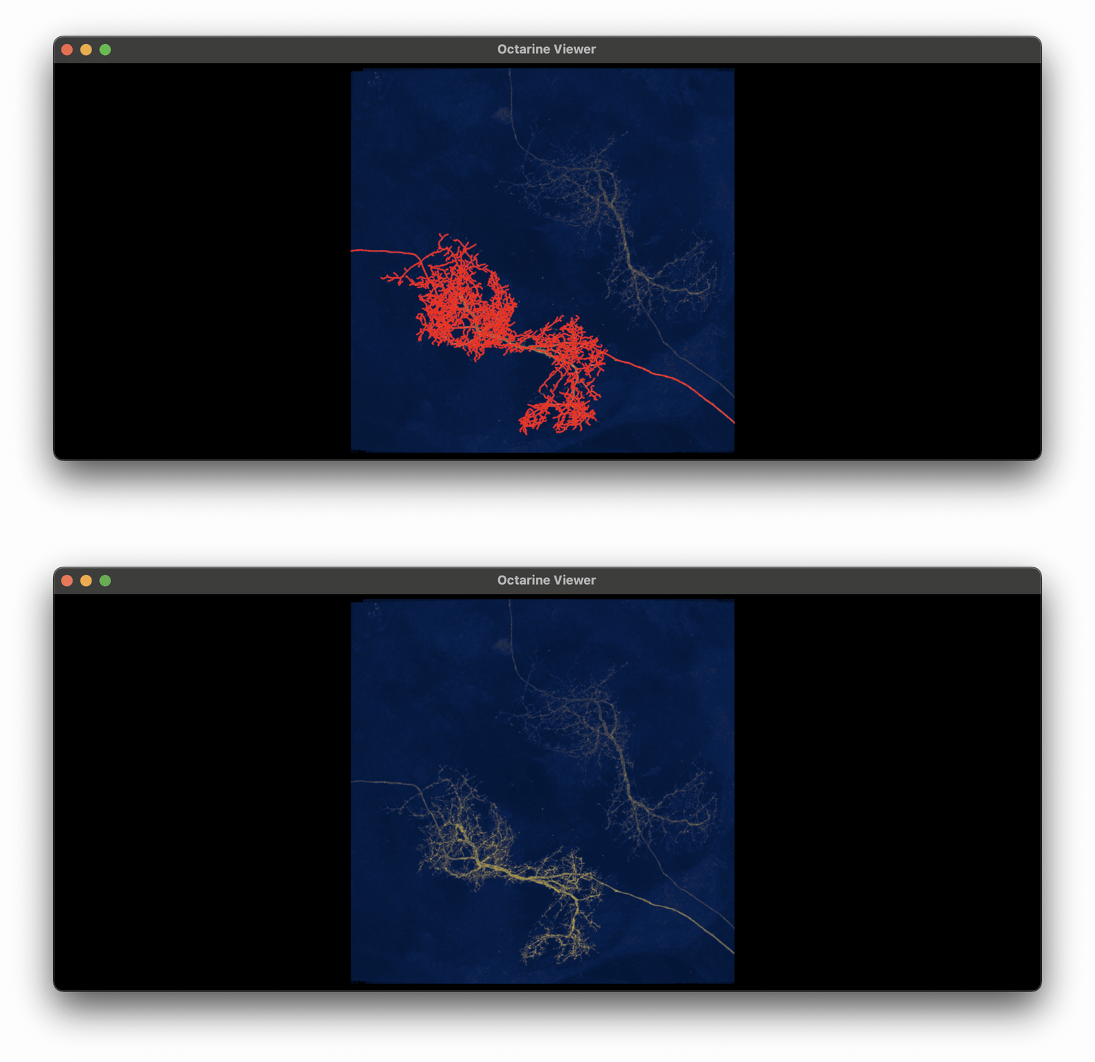
This looks pretty good off the bat! Now obviously we will have the other large neuron (label 6091) plus bunch of smaller skeletons in our NeuronList. Let's have a look at those as well:

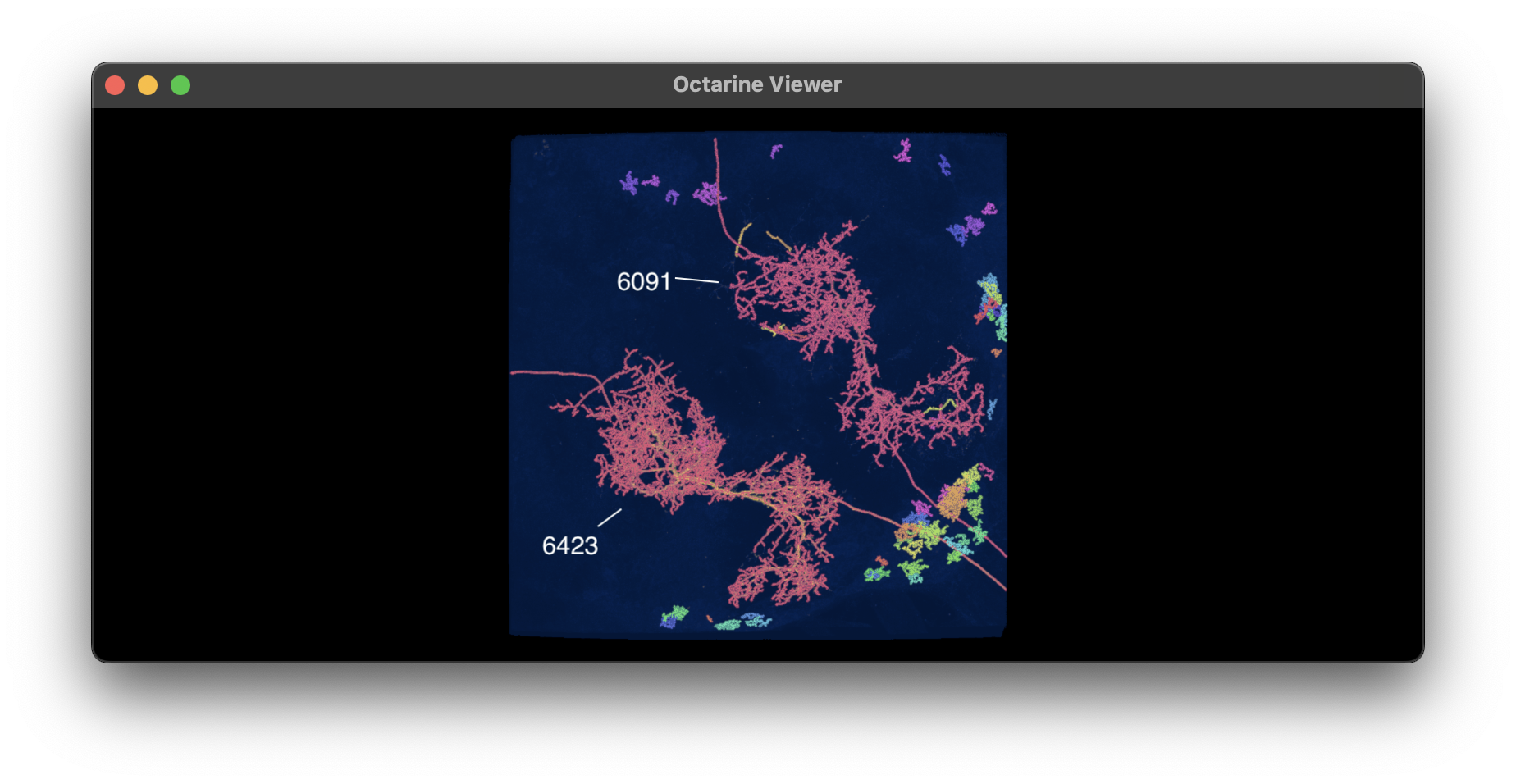
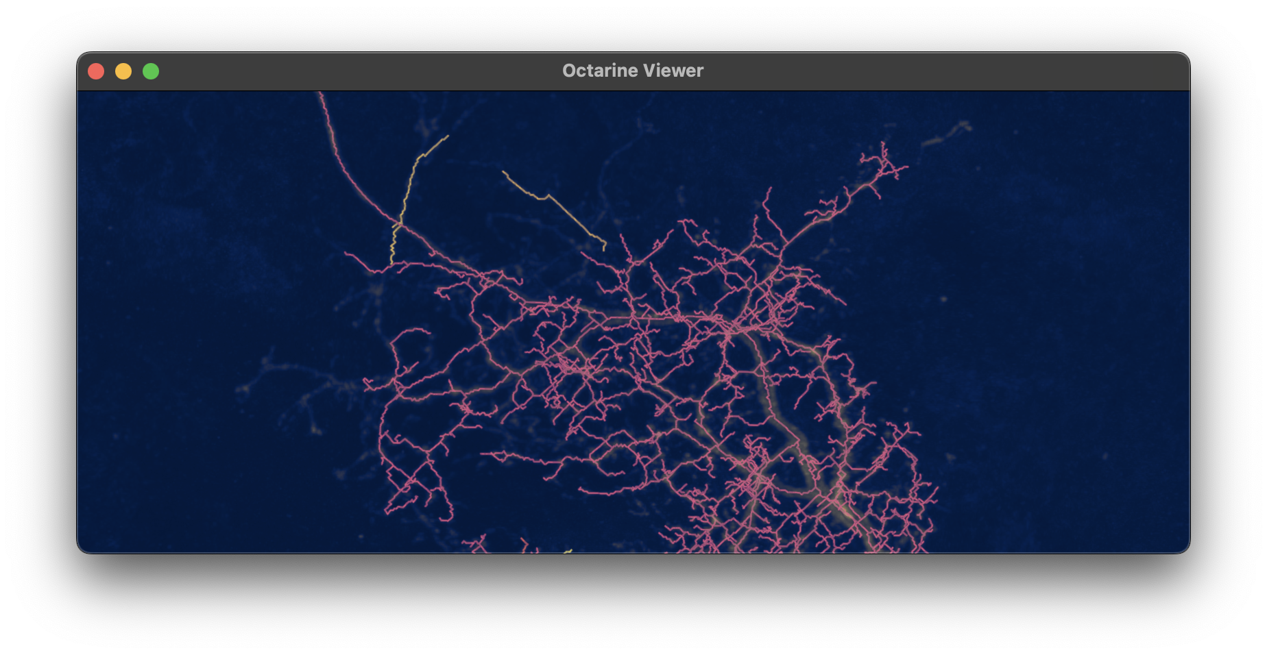
Zooming in on 6091 you will see that it wasn't fully skeletonized: some of the branches are missing and others are disconnected. That's either because our threshold for the mask was too high (this neuron had a weaker signal than the other) and/or we dropped too many fragments during the skeletonization process (see the dust_threshold parameter).

Alternatives

If this pipeline doesn't work for your data, consider:

Tool	What it is
Simple Neurite Tracer	Popular ImageJ plugin for semi-automated tracing.
Vaa3D / Mozak	The Allen Institute's protocol for reconstructing neurons.
NeuTube	Open-source reconstruction from fluorescence microscopy images.

Acknowledgements

The packages we used here were written by the excellent Will Silversmith from the Seung lab in Princeton. The image stack we processed is from the Janelia Split-Gal4 collection and was published as part of the Cheong, Eichler, Stuerner, et al. (2024) paper.

Total running time of the script: ( 0 minutes 0.000 seconds)

Download Python source code: zzz_tutorial_io_05_skeletonize.py

Download Jupyter notebook: zzz_tutorial_io_05_skeletonize.ipynb

Gallery generated by mkdocs-gallery