Volumes#

Give a figure context without letting the neuropil steal it.

Volumes - neuropils, brain outlines, ROIs - are meshes, so most of what the mesh tutorial says applies here too. What makes them their own topic is their job: a neuropil is scenery. It has to say "here is where we are" and then get out of the way of the neuron you actually want people to look at.

NAVis treats them accordingly. A volume always sits at the very bottom of the stack, never joins the depth bins and never takes a halo - so you can hand plot2d a mixed scene and not think about ordering.

Parameter	Effect
`color` / `alpha`	As for any object; volumes carry a default colour of their own
`volume_outlines`	Draw a contour instead of a surface (`True`), or both (`"both"`)
`volume_outlines_alpha`	Alpha-shape tightness for that contour; default `0.001`
`mesh_shade`	Light the surface - `"ghost"` is the interesting one here

The default: a translucent surface#

Volumes come with their own colour and alpha (a pale grey at 20% for the example volumes), so passing one straight to plot2d already gives you something usable:

import navis
import matplotlib.pyplot as plt

n = navis.example_neurons(1, kind="skeleton")
lh = navis.example_volume("LH")

fig, ax = navis.plot2d([n, lh], view=("x", "-z"), method="2d")
plt.tight_layout()

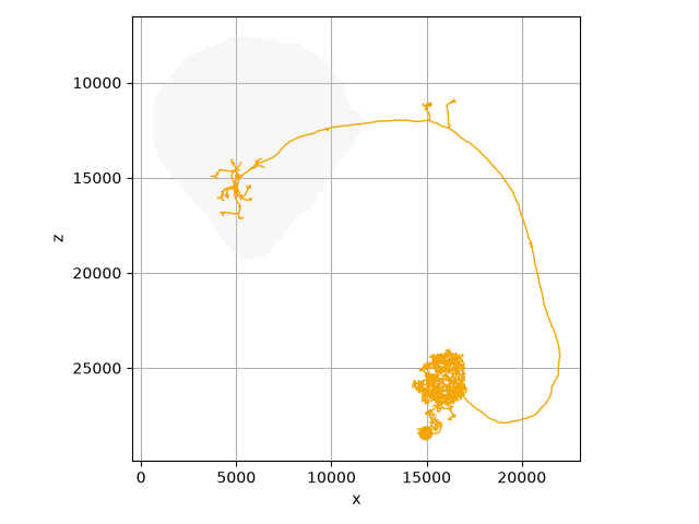
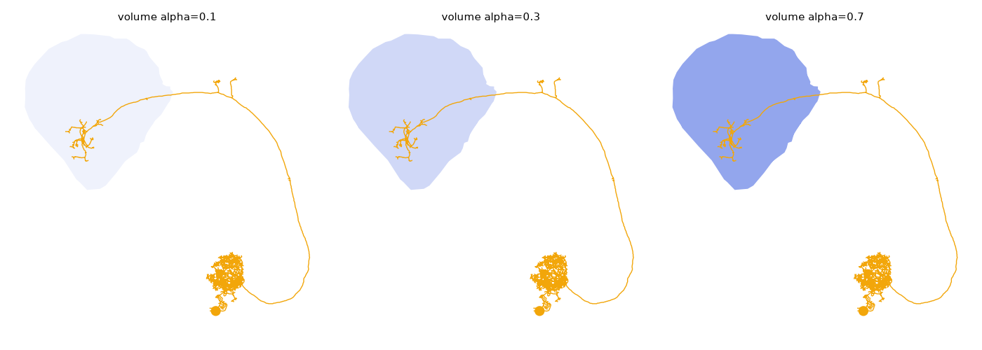
The alpha is worth a note. A neuropil is nearly always translucent, and translucency is exactly the case a per-face renderer gets wrong: every triangle composites separately, so the surface reads as its own triangulation and folds come out darker than flat stretches. NAVis fills the union of the visible faces as a single path instead, so alpha means what it says:

fig, axes = plt.subplots(1, 3, figsize=(14, 5))
for ax, alpha in zip(axes, [0.1, 0.3, 0.7]):
    navis.plot2d([n, lh], ax=ax, method="2d", view=("x", "-z"), color={lh.name: (0.4, 0.5, 0.9, alpha)})
    ax.set_title(f"volume alpha={alpha}", fontsize=11, y=0.98)
    ax.set_axis_off()
plt.tight_layout()

Outlines instead of surfaces#

volume_outlines=True swaps the filled surface for a single contour - the cheapest possible way to give a figure context, and often the most legible:

fig, axes = plt.subplots(1, 3, figsize=(14, 5))
for ax, outlines in zip(axes, [False, True, "both"]):
    navis.plot2d([n, lh], ax=ax, method="2d", view=("x", "-z"), volume_outlines=outlines)
    ax.set_title(f"volume_outlines={outlines!r}", fontsize=11, y=0.98)
    ax.set_axis_off()
plt.tight_layout()

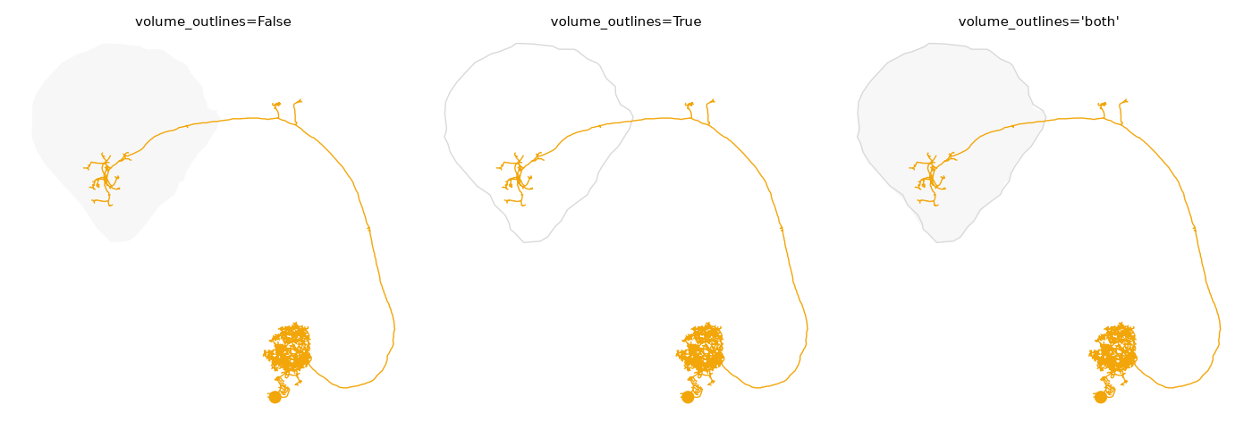
The contour is always drawn opaque, whatever alpha the volume carries. A volume's alpha is a fill alpha - it is there so you can see the neuron through the neuropil - and there is nothing to see through a line, so at the 10-20% volumes default to it would simply be invisible.

Outlines need shapely

The contour is an alpha shape of the projected vertices, which NAVis computes with shapely. Install it (pip install shapely) or you will get an error.

volume_outlines_alpha controls how tightly that shape wraps the projection: near zero gives you the convex hull, larger values let it follow concavities. On the whole-brain outline the difference is the difference between a blob and a fly brain:

brain = navis.example_volume("neuropil")

fig, axes = plt.subplots(1, 4, figsize=(17, 5))
for ax, a in zip(axes, [0.00001, 0.0001, 0.0003, 0.001]):
    navis.plot2d(
        brain, ax=ax, method="2d", view=("x", "-z"), color=(0.2, 0.3, 0.7),
        volume_outlines=True, volume_outlines_alpha=a,
    )
    ax.set_title(f"volume_outlines_alpha={a}", fontsize=11, y=0.98)
    ax.set_axis_off()
plt.tight_layout()

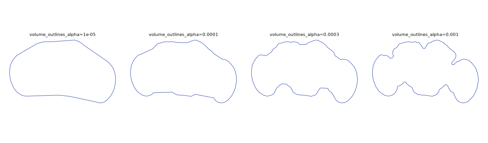
The useful range depends on the mesh

alpha is a radius filter in data units: a triangle survives if its circumradius is below 1/alpha. The useful range therefore scales with your coordinate system, and no single value is right for every volume. 10 / (size of the volume) is a decent starting guess - which is where the default of 0.001 comes from, since these example meshes are ~10,000 units across.

Push it too far and the shape breaks into disconnected pieces. NAVis then retries at a tenth of the alpha and warns you - so if a large value seems to have no effect, check the log: it was probably rolled back.

Ghost shading#

The awkward thing about a filled neuropil is the choice it forces: opaque enough to read as a solid, or transparent enough to see the neuron inside. mesh_shade="ghost" sidesteps it by taking opacity from the grazing angle - dense where the surface turns away from you, clear where it faces you:

fig, axes = plt.subplots(1, 3, figsize=(14, 5))
for ax, (title, kwargs) in zip(
    axes,
    [
        ("flat", dict()),
        ("mesh_shade=True", dict(mesh_shade=True)),
        ('mesh_shade="ghost"', dict(mesh_shade="ghost")),
    ],
):
    navis.plot2d([n, lh], ax=ax, method="2d", view=("x", "-z"), **kwargs)
    ax.set_title(title, fontsize=11, y=0.98)
    ax.set_axis_off()
plt.tight_layout()

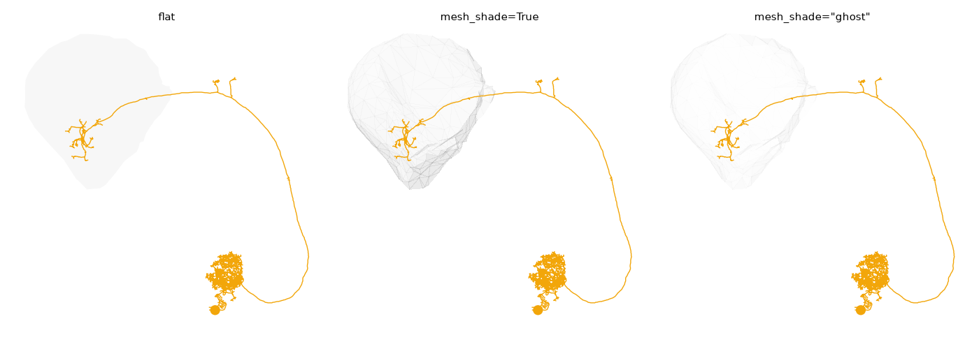
Look closely at the middle panel: plain mesh_shade=True needs one polygon per face, and on a translucent mesh that means every triangle composites on its own - so the 756-face LH shows its own wireframe. "ghost" varies alpha rather than brightness and reads far more cleanly. strength scales the term:

navis.plot2d(lh, mesh_shade={"mode": "ghost", "strength": 1.8})

Volumes are always scenery#

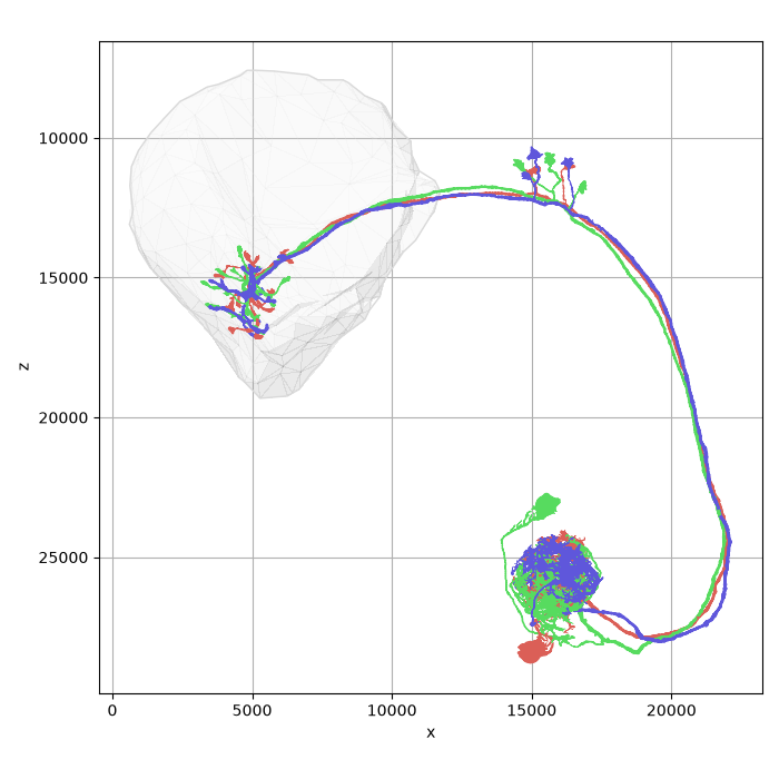
Three deliberate asymmetries between volumes and mesh neurons, all of them so that a mixed scene does the right thing without being told:

	Mesh neuron	Volume
z-order	above skeletons by default	always at the bottom
`depth_sort`	joins the stack	stays out of it
`halo`	gets one	never

Which means this is all you need for a figure with context:

nl = navis.example_neurons(3, kind="skeleton")

fig, ax = navis.plot2d(
    [nl, lh],
    view=("x", "-z"),
    method="2d",
    style="publication",
    volume_outlines="both",
    figsize=(7, 7),
)
plt.tight_layout()

Several volumes at once#

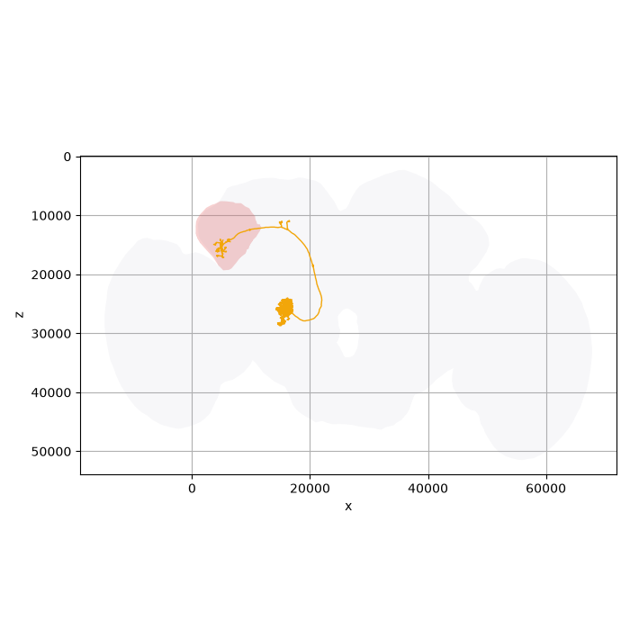
Colour them the way you would any other object - a list, or a dict keyed by name:

fig, ax = navis.plot2d(
    [n, lh, brain],
    view=("x", "-z"),
    method="2d",
    color={lh.name: (0.9, 0.4, 0.4, 0.3), brain.name: (0.6, 0.6, 0.7, 0.08)},
    figsize=(7, 7),
)
plt.tight_layout()

Volumes of your own

Anything you can turn into a navis.Volume works here - a .obj file, a trimesh.Trimesh, or vertices and faces you built yourself. See the mesh I/O tutorial.

Total running time of the script: ( 0 minutes 5.526 seconds)

Download Python source code: tutorial_plotting_2d_02_volumes.py

Download Jupyter notebook: tutorial_plotting_2d_02_volumes.ipynb

Gallery generated by mkdocs-gallery