Note
Click here to download the full example code
Connectors#
Show where a neuron talks to its partners.
A neuron's connectors are its synapses, gap junctions - anything with a position on the neuron and a type. Any neuron that carries a connectors table can draw them, whatever its class, and every backend understands the same set of cn_* parameters.
The table itself is a plain pandas.DataFrame, which turns out to be the most important thing about it: half of what follows is really about filtering a DataFrame before handing it to a plotting function.
| Parameter | Effect | plot2d | plot3d |
|---|---|---|---|
connectors | Which connectors to draw - all, or a subset by type | ||
connectors_only | Draw the connectors but not the neuron | ||
cn_colors | One colour, a colour per type, or "neuron" | ||
cn_color_by | Colour by any other column of the connector table | plotly, k3d | |
cn_palette | Palette for cn_color_by | plotly, k3d | |
cn_size | Marker size | ||
cn_alpha | Marker transparency | ||
cn_layout | Per-type names/colours, and display (see below) | ||
cn_legend | A legend entry per type, or a colorbar | ||
cn_zorder | Where connectors sit in the stack |
What is in a connector table#
The example neurons ship with one, so there is nothing to fetch:
import navis
import pandas as pd
import matplotlib.pyplot as plt

n = navis.example_neurons(1, kind="skeleton")
n.connectors.head()
x/y/z is where it sits, node_id is the node it belongs to, and type is what everything below keys off. These particular connectors also carry a roi and a confidence, which is typical - what columns you get depends on where the data came from.
Every backend draws them#
connectors=True is all it takes, in plot2d (both its flat and its matplotlib 3D modes) and in plot3d (octarine, plotly and k3d alike):
fig = plt.figure(figsize=(15, 5))

ax = fig.add_subplot(1, 3, 1)
navis.plot2d(n, ax=ax, method="2d", view=("x", "-z"), color="lightgrey",
             connectors=True, cn_size=6)
ax.set_title('plot2d, method="2d"', fontsize=11, y=0.98)
ax.set_axis_off()

ax = fig.add_subplot(1, 3, 2, projection="3d")
navis.plot2d(n, ax=ax, method="3d", view=("x", "-z"), color="lightgrey",
             connectors=True, cn_size=6)
ax.set_title('plot2d, method="3d"', fontsize=11, y=0.98)
ax.set_xticks(ax.get_xticks()[::2])  # a 3d axis is drawn small inside its slot
ax.tick_params(labelsize=8)

ax = fig.add_subplot(1, 3, 3)
navis.plot3d(n, snapshot=True, ax=ax, view=("x", "-z"), color="lightgrey",
             connectors=True, cn_size=3)
ax.set_title("plot3d, octarine snapshot", fontsize=11, y=0.98)
ax.set_axis_off()

plt.tight_layout()
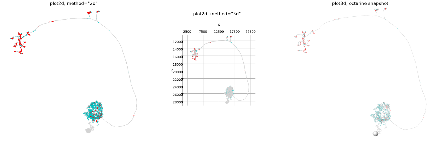
Red is presynaptic (this neuron's output), cyan postsynaptic (its input) - the defaults live in navis.config.default_connector_colors. The rest of this page uses plot2d(method="2d") for the comparisons, because it is the cheapest way to put settings side by side; everything except cn_zorder applies just as well to the others.
Which connectors#
connectors doubles as the filter. True draws all of them, "pre"/"presynapses" and "post"/"postsynapses" are shorthands, and anything else is matched against the type column - either a single value or a list of them:
fig, axes = plt.subplots(1, 3, figsize=(15, 5))
for ax, which in zip(axes, [True, "pre", "post"]):
    navis.plot2d(n, ax=ax, method="2d", view=("x", "-z"), color="lightgrey",
                 connectors=which, cn_size=6)
    ax.set_title(f"connectors={which!r}", fontsize=11, y=0.98)
    ax.set_axis_off()
plt.tight_layout()
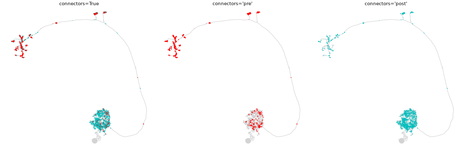
That already tells you something: the inputs (right) are almost all in the dense lower arbour, the outputs (middle) mostly in the upper two. This is an olfactory projection neuron, and the picture is close to the definition of one. Since this table also carries an roi, we can check that rather than eyeball it:
pd.crosstab(n.connectors.roi, n.connectors.type)
93% of the postsynapses are in the antennal lobe, and the presynapses split between the lateral horn and the calyx - with a substantial minority back in the AL. Worth noticing, because the middle panel above rather undersells that minority; we come back to why below.
type is whatever your data says
"pre"/"post" are conventions, not requirements. If your connector table uses 0/1, or "chemical"/"electrical", pass those instead - connectors="chemical" filters the column directly. Only the default colours know about the usual names.
Colours#
cn_colors takes a single colour for everything, a dict keyed by type, or "neuron" to make the connectors match the neuron they belong to:
fig, axes = plt.subplots(1, 3, figsize=(15, 5))
for ax, (title, kwargs) in zip(
    axes,
    [
        ("cn_colors='k'", dict(cn_colors="k")),
        ("cn_colors={'pre': ...}", dict(cn_colors={"pre": "magenta"})),
        ("cn_colors='neuron'", dict(cn_colors="neuron")),
    ],
):
    navis.plot2d(n, ax=ax, method="2d", view=("x", "-z"), color="darkorange",
                 connectors=True, cn_size=6, **kwargs)
    ax.set_title(title, fontsize=11, y=0.98)
    ax.set_axis_off()
plt.tight_layout()
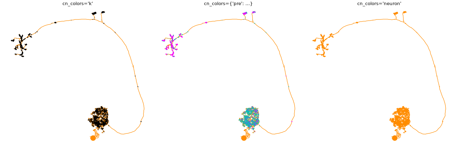
A dict only has to cover the types you care about - the middle panel recolours "pre" and leaves "post" on its default. cn_colors="neuron" is the one to reach for when the neuron, not the synapse type, is what a reader needs to tell apart; it is the same thing as cn_mesh_colors=True.
Size and transparency#
The default marker is deliberately tiny, which is the wrong choice as soon as you have a few thousand of them in one arbour. cn_size and cn_alpha are how you get a readable density:
fig, axes = plt.subplots(2, 2, figsize=(11, 10))
for ax, (title, kwargs) in zip(
    axes.flat,
    [
        ("default", dict()),
        ("cn_size=10", dict(cn_size=10)),
        ("cn_size=30", dict(cn_size=30)),
        ("cn_size=30, cn_alpha=0.15", dict(cn_size=30, cn_alpha=0.15)),
    ],
):
    navis.plot2d(n, ax=ax, method="2d", view=("x", "-z"), color="lightgrey",
                 connectors=True, **kwargs)
    ax.set_title(title, fontsize=11, y=0.98)
    ax.set_axis_off()
plt.tight_layout()
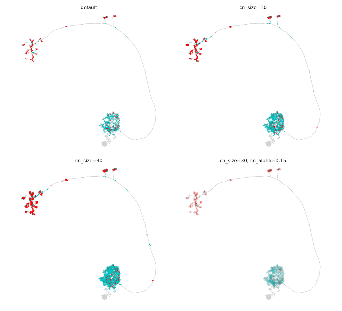
Big and opaque (bottom left) turns the antennal lobe into one solid disc - you can see that there are synapses, not how many. Big and translucent (bottom right) reads as density instead: the darker the patch, the more synapses stacked on it.
Why the antennal lobe reads cyan
Whichever type is drawn last wins wherever markers overlap. Painting one type after another would therefore let a rare type bury a common one - here 232 presynapses would sit on top of 1933 postsynapses and the antennal lobe would read as an output region, which it is not.
So NAVis puts all of a neuron's connectors into a single artist and draws them in a shuffled order. The mix you see is then a fair sample of the real one: the AL comes out mostly cyan because it mostly is postsynaptic. The shuffle is seeded, so the same data always gives the same figure.
cn_alpha is still worth reaching for when the exact ratio matters - overlapping markers hide each other however they are ordered.
cn_size is not one unit
Each backend passes it to its own renderer, so the same number means different things: matplotlib reads it as a marker area in points², plotly as a diameter in pixels, and k3d and octarine as a size in world units. Expect to retune it when you switch backends.
Where connectors sit in the stack#
By default connectors are drawn above everything else, so a synapse is never hidden by the neurite it sits on. cn_zorder overrides that - useful when the neuron is the subject and the synapses are context:
nl = navis.example_neurons(3, kind="skeleton")

fig, axes = plt.subplots(1, 2, figsize=(11, 5.5))
for ax, z in zip(axes, [None, 0]):
    navis.plot2d(nl, ax=ax, method="2d", view=("x", "-z"), radius=True,
                 connectors="pre", cn_size=25, cn_alpha=0.5, cn_zorder=z)
    ax.set_title(f"cn_zorder={z!r}", fontsize=11, y=0.98)
    ax.set_axis_off()
plt.tight_layout()
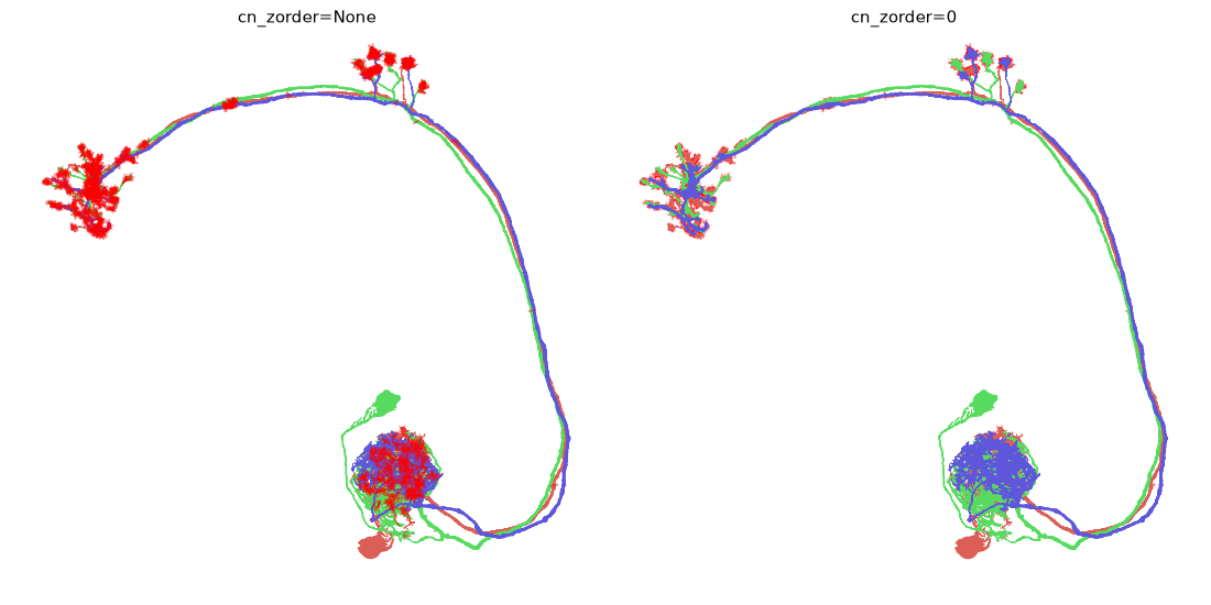
cn_zorder is a plot2d-only setting - the 3D backends resolve occlusion properly and have nothing to override.
Connectors on their own#
connectors_only=True drops the neuron and keeps the synapses. Paired with a second, greyed-out call it gives you a synapse cloud in anatomical context:
fig, ax = plt.subplots(figsize=(7, 7))

# the skeletons, as scenery
navis.plot2d(nl, ax=ax, method="2d", view=("x", "-z"), color=(0, 0, 0, 0.12), linewidth=1)
# the synapses, on top
navis.plot2d(nl, ax=ax, method="2d", view=("x", "-z"),
             connectors_only=True, connectors="pre", cn_colors="crimson",
             cn_size=25, cn_alpha=0.4)
ax.set_axis_off()
plt.tight_layout()
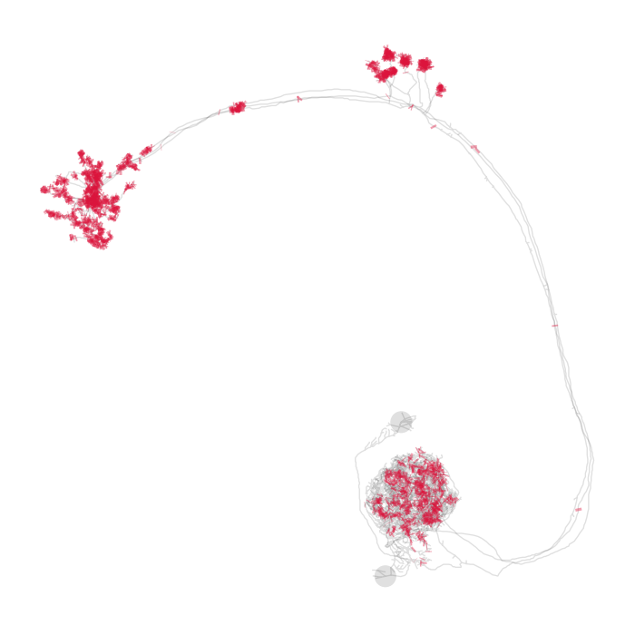
Legends#
cn_legend=True adds one entry per connector type - per type, not per type per neuron, which is why it is a separate switch rather than a label on the artists. Call ax.legend() afterwards as usual:
fig, ax = navis.plot2d(n, method="2d", view=("x", "-z"), color="lightgrey",
                       connectors=True, cn_size=8, cn_legend=True, figsize=(7, 7))
ax.legend(loc="upper right", frameon=False)
ax.set_axis_off()
plt.tight_layout()
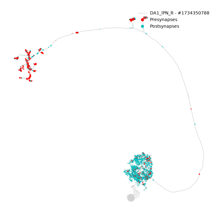
The labels come from navis.config.default_connector_colors, so renaming a type there - or via cn_layout - renames it in the legend too.
Colouring by anything else#
cn_colors keys off the type column. cn_color_by takes any other column instead - or an array with one value per connector - and cn_palette says how to colour it. Categorical data gets one colour per level and a legend:
fig, ax = navis.plot2d(
    n, method="2d", view=("x", "-z"), color="lightgrey", figsize=(7, 7),
    connectors=True, cn_size=14, cn_alpha=0.7,
    cn_color_by="roi", cn_palette="tab10", cn_legend=True,
)
ax.legend(loc="upper right", frameon=False)
ax.set_axis_off()
plt.tight_layout()
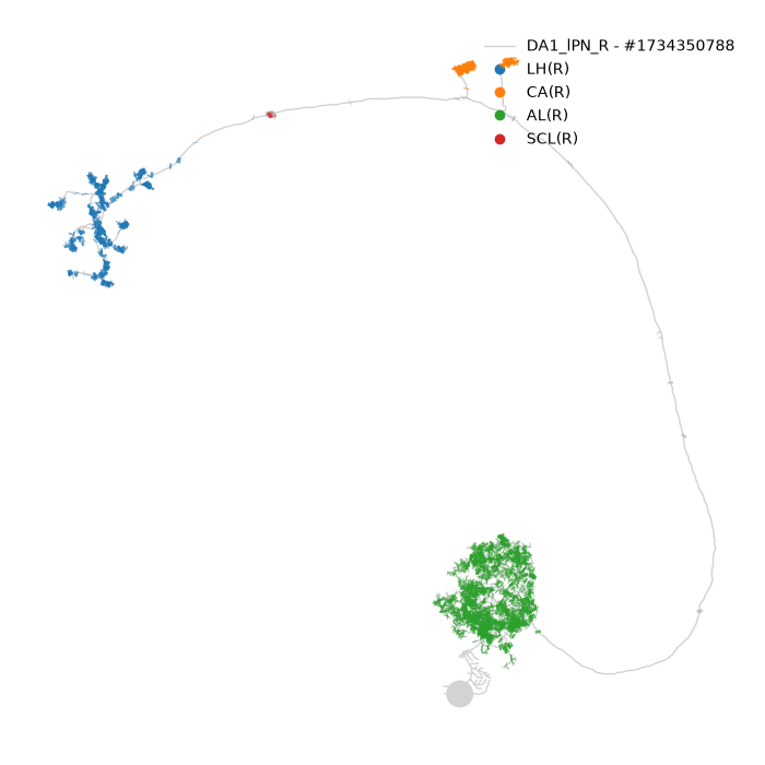
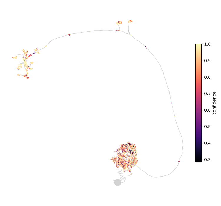
Numerical data gets a colormap and, with cn_legend=True, a colorbar - there is no finite set of entries a legend could list:
fig, ax = navis.plot2d(
    n, method="2d", view=("x", "-z"), color="lightgrey", figsize=(7.5, 7),
    connectors=True, cn_size=14,
    cn_color_by="confidence", cn_palette="magma", cn_legend=True,
)
ax.set_axis_off()
plt.tight_layout()
One scale for all neurons
The colour scale is worked out across every neuron in the call, so the same value is the same colour throughout - which is the whole point of a shared legend. Connectors whose value is missing are drawn grey and left out of the legend.
The table is just a DataFrame#
connectors and cn_color_by between them cover most of what you would want, but neither filters on anything except type. For that, hand the neuron a smaller table:
confident = n.copy()
confident.connectors = n.connectors[n.connectors.confidence > 0.99].copy()
navis.plot2d(confident, connectors=True)
Work on a copy
n.copy() there is not decoration. Assigning to n.connectors would mutate the neuron for the rest of the session - and copying is cheap next to a plot.
Stalks instead of dots#
cn_layout carries the per-type names and colours plus display, which decides what a connector actually looks like. "lines" - the default - draws a stalk from each connector back to the node it belongs to; "circles" draws a free-floating marker. At whole-cell zoom the two are hard to tell apart, so here is a crop of the lateral horn:
fig, axes = plt.subplots(1, 2, figsize=(11, 5.5))
for ax, display in zip(axes, ["lines", "circles"]):
    navis.plot2d(n, ax=ax, method="2d", view=("x", "-z"), color="lightgrey",
                 connectors=True, cn_size=8, cn_layout={"display": display})
    ax.set_title(f'display="{display}"', fontsize=11, y=0.98)
    ax.set_xlim(3500, 7500)
    ax.set_ylim(18000, 13000)
    ax.set_axis_off()
plt.tight_layout()
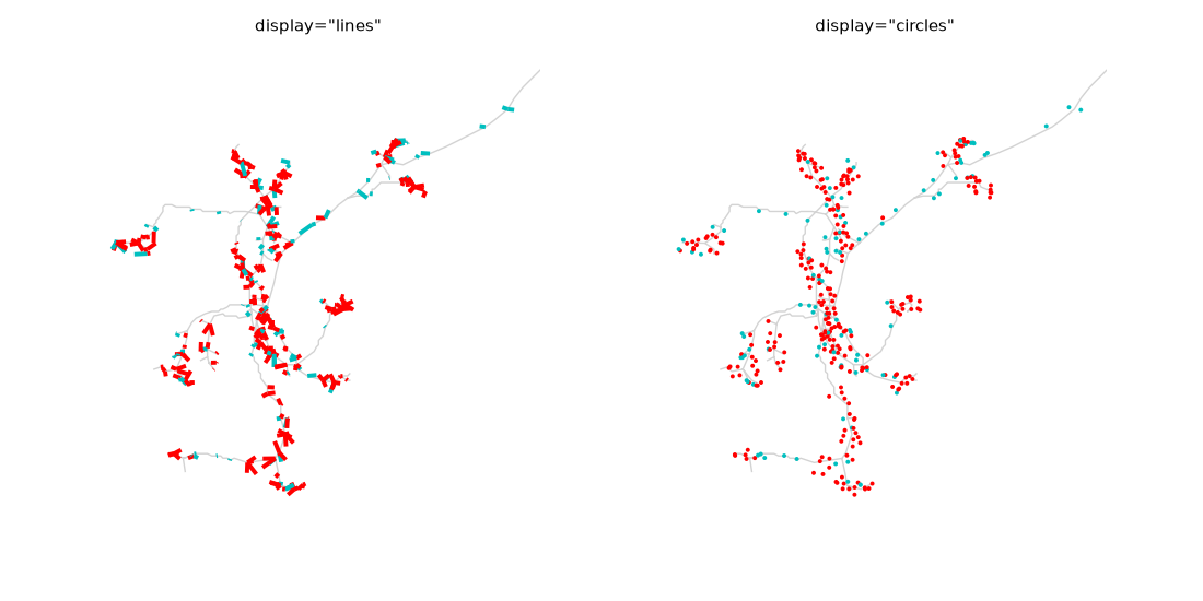
The stalk is worth having wherever synapses sit off the skeleton, which is common in EM data: it tells you which neurite a synapse belongs to instead of leaving you to guess from proximity. It needs a node to point at, so meshes - which have none - always get circles.
cn_layout also renames and recolours types wholesale, which is the tidier route when you want one scheme across a whole figure:
navis.plot3d(
    n,
    backend="plotly",
    connectors=True,
    cn_layout={
        "display": "circles",
        "size": 3,
        "pre": {"name": "output", "color": (1, 0.3, 0)},
        "post": {"name": "input", "color": (0.1, 0.4, 0.9)},
    },
)
Here it is live in plotly, stalks and all:
navis.plot3d(n, backend="plotly", connectors=True, color="lightgrey",
             legend=False, height=600)
Several neurons#
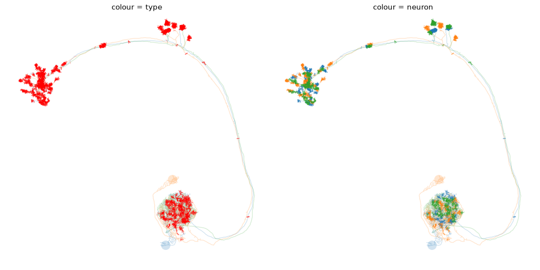
Everything above works unchanged on a NeuronList. The one decision worth making deliberately is what the colour should mean - the synapse type, or the neuron:
fig, axes = plt.subplots(1, 2, figsize=(11, 5.5))
for ax, (title, kwargs) in zip(
    axes,
    [
        ("colour = type", dict()),
        ("colour = neuron", dict(cn_colors="neuron")),
    ],
):
    navis.plot2d(nl, ax=ax, method="2d", view=("x", "-z"), palette="tab10", alpha=0.2,
                 connectors="pre", cn_size=18, cn_alpha=0.6, **kwargs)
    ax.set_title(title, fontsize=11, y=0.98)
    ax.set_axis_off()
plt.tight_layout()
Where next
Connectors are only the positions - what a plot can show you is where a neuron receives and where it sends. For what they are actually used for, see the axon-dendrite split, which is driven entirely by this table.
Total running time of the script: ( 0 minutes 4.018 seconds)
Download Python source code: tutorial_plotting_misc_00_connectors.py
Download Jupyter notebook: tutorial_plotting_misc_00_connectors.ipynb