Meshes#

Light mesh neurons properly - which is what a real renderer is for.

A Mesh is a surface, and a surface is where 3D earns its keep: the renderer does occlusion and lighting for you, so none of the 2D machinery - culling, depth sorting, mesh_shade modes - is needed here.

What you get instead is control over the lighting model, and that lives mostly in the plotly backend. If you have not read the plotting overview yet, start there.

Parameter	Effect	octarine	plotly	k3d
`color`/`alpha`	As everywhere else
`color_by`	Per-vertex colours
`lighting`	Lighting preset or an explicit dict
`lightposition`	Where the key light sits
`flatshading`	Faceted, low-poly look
`snapshot`	Render offscreen into a `matplotlib` figure

The interactive viewer#

Mesh neurons need no setup - hand one to plot3d and the renderer takes care of the rest. Drag the figure below to rotate it and watch the highlight track the surface:

import navis
import matplotlib.pyplot as plt

m = navis.example_neurons(1, kind="mesh")

navis.plot3d(m, backend="plotly", lighting="glossy", color="#4C6EF5", legend=False, height=550)

Lighting presets (plotly)#

That was the "glossy" preset. Plotly's own mesh defaults are washed out - ambient=0.8 with almost no specular, so a surface comes out nearly flat - and NAVis ships presets that fix that, selectable by name:

Preset	Look
`True` / `"default"` / `"studio"`	Dimensional but not shiny. The default
`"matte"`	Soft, no highlights - good for busy scenes
`"glossy"`	Wet/plastic, strong highlights
`"rim"`	Bright rim - reads well on translucent shells
`False` / `"plotly"`	Plotly's own near-flat defaults

Pass a dict to set ambient, diffuse, specular, roughness and fresnel yourself:

navis.plot3d(m, backend="plotly", lighting="matte")
navis.plot3d(m, backend="plotly", lighting={"ambient": 0.3, "specular": 0.9})

Two companions to lighting:

lightposition - a dict with x/y/z. By default NAVis derives it from each mesh's bounding box, so the key light is always sensibly placed.
flatshading - True shades each face by its own normal instead of interpolating, which gives a deliberately faceted, low-poly look.

navis.plot3d(m, backend="plotly", flatshading=True)
navis.plot3d(m, backend="plotly", lightposition={"x": 1e5, "y": 1e5, "z": 1e5})

Snapshots#

snapshot=True renders the octarine scene offscreen onto a matplotlib axes - which is what lets the rest of this page put settings side by side. Compare it with the flat 2D version and it is obvious what a renderer buys you: the tubes read as tubes rather than as a silhouette, without anything being switched on.

fig, axes = plt.subplots(1, 2, figsize=(11, 5.5))
navis.plot2d(m, ax=axes[0], method="2d", view=("x", "-z"), color="#4C6EF5")
axes[0].set_title("plot2d, flat", fontsize=11, y=0.98)
navis.plot3d(m, snapshot=True, ax=axes[1], view=("x", "-z"), color="#4C6EF5")
axes[1].set_title("plot3d, snapshot", fontsize=11, y=0.98)
for ax in axes:
    ax.set_axis_off()
plt.tight_layout()

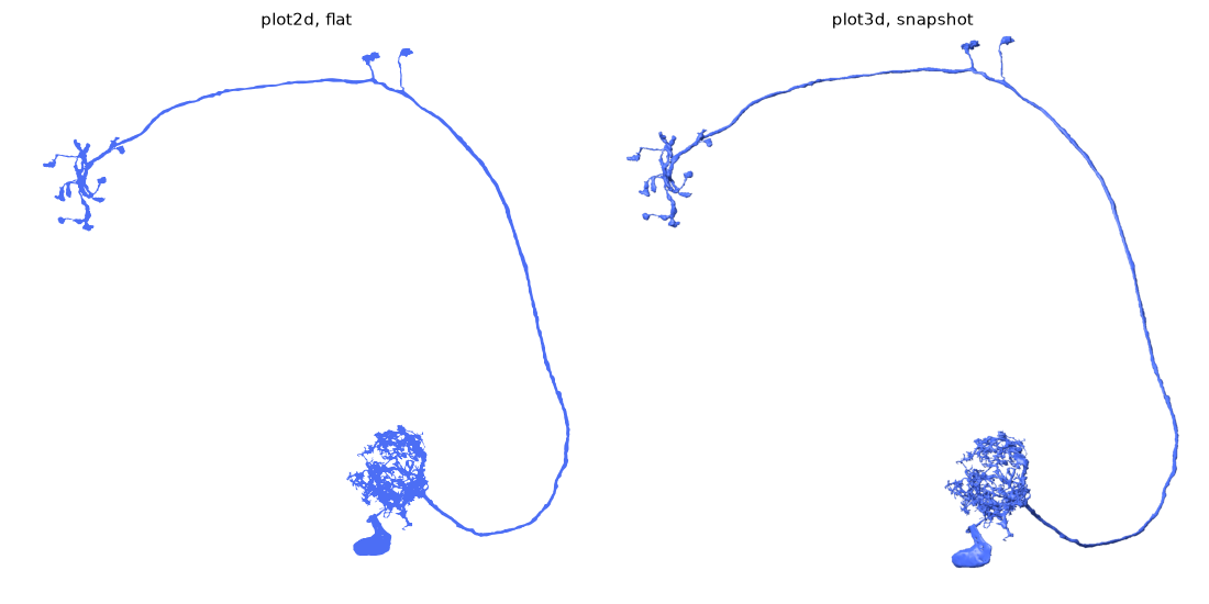
2D can get close

plot2d(..., mesh_shade=True) does its own Lambertian shading and gets a good way there at a fraction of the cost, in vector output. See 2D meshes.

Snapshots use octarine, so lighting does not apply

The presets above are a plotly feature. A snapshot is octarine's renderer, which lights the scene its own way - so the panels below differ in colour and alpha, not in lighting model.

Colours and transparency#

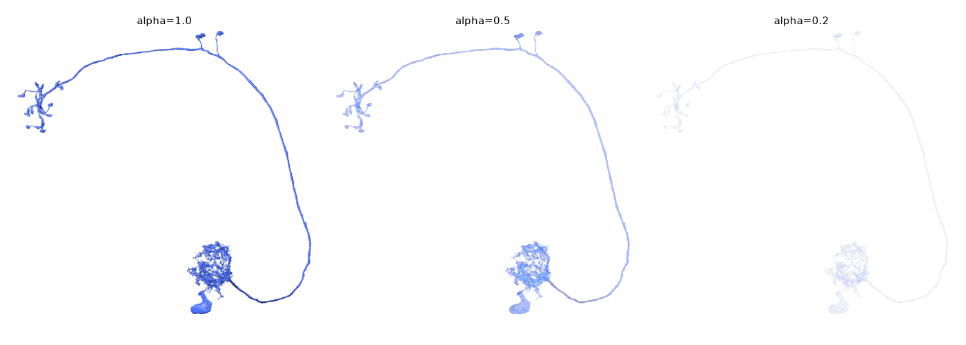
color, alpha, color_by and palette behave exactly as they do everywhere else - see coloring. Alpha is worth showing though, because a real renderer composites it correctly no matter how the surface folds:

fig, axes = plt.subplots(1, 3, figsize=(14, 5))
for ax, alpha in zip(axes, [1.0, 0.5, 0.2]):
    navis.plot3d(m, snapshot=True, ax=ax, view=("x", "-z"), color="#4C6EF5", alpha=alpha)
    ax.set_title(f"alpha={alpha}", fontsize=11, y=0.98)
    ax.set_axis_off()
plt.tight_layout()

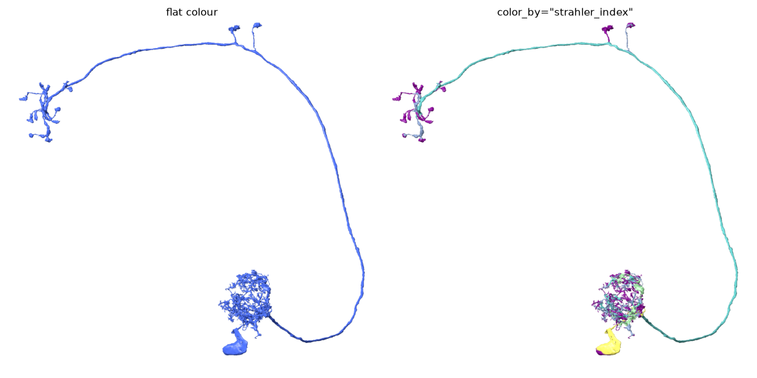
And per-vertex colouring, which shading multiplies into rather than replacing:

fig, axes = plt.subplots(1, 2, figsize=(11, 5.5))
navis.plot3d(m, snapshot=True, ax=axes[0], view=("x", "-z"), color="#4C6EF5")
axes[0].set_title("flat colour", fontsize=11, y=0.98)
navis.plot3d(
    m, snapshot=True, ax=axes[1], view=("x", "-z"),
    color_by="strahler_index", palette="viridis",
)
axes[1].set_title('color_by="strahler_index"', fontsize=11, y=0.98)
for ax in axes:
    ax.set_axis_off()
plt.tight_layout()

Several meshes#

Occlusion between neurons is simply correct - no depth_sort, no bins, nothing to tune:

nl = navis.example_neurons(3, kind="mesh")

fig, axes = plt.subplots(1, 2, figsize=(11, 5.5))
navis.plot2d(nl, ax=axes[0], method="2d", view=("x", "-z"), depth_sort="global")
axes[0].set_title('plot2d, depth_sort="global"', fontsize=11, y=0.98)
navis.plot3d(nl, snapshot=True, ax=axes[1], view=("x", "-z"))
axes[1].set_title("plot3d, snapshot", fontsize=11, y=0.98)
for ax in axes:
    ax.set_axis_off()
plt.tight_layout()

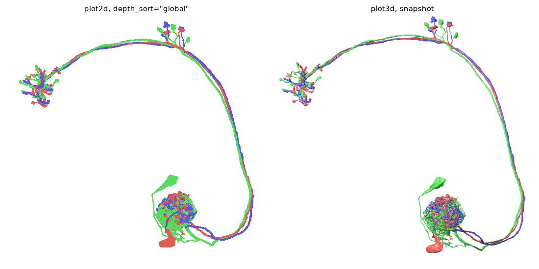
That comparison is the short version of the whole 2D/3D trade-off: the left panel is vector output you can edit in Illustrator and cost NAVis a great deal of machinery to get right; the right panel is a raster image that came out correct for free.

Neuropils

Volumes are meshes too, but translucent shells have their own problems and their own settings - see 3D volumes.

Total running time of the script: ( 0 minutes 4.726 seconds)

Download Python source code: tutorial_plotting_3d_01_meshes.py

Download Jupyter notebook: tutorial_plotting_3d_01_meshes.ipynb

Gallery generated by mkdocs-gallery