"""
IVSCC morphometrics
===================
Measure cortical neurons compartment by compartment.
!!! important "This example is not executed"
Like the [skeleton QC tutorial](zzz_tutorial_morpho_04_qc), this one is *not* run when the docs are
built - it pulls ~25 reconstructions from a remote repository, which is not something to lean on in
CI. The code is real and runnable; the outputs and plots shown here are statically embedded.
Most morphometrics treat a neuron as one undifferentiated tree. For a **cortical** neuron that throws away
the most informative thing about it: a layer-5 pyramidal cell is not "a tree with 800 µm of reach", it is a
*basal* bush around the soma, an *apical* trunk climbing to the pia, and an *axon* heading the other way.
The three answer different questions and have to be measured separately.
[`navis.ivscc_features`][] does exactly that. It follows the feature set from the Allen Institute's
IVSCC pipeline: split the neuron on its compartment labels, measure each part on its own, then add a
handful of features describing how the parts relate to the soma and to each other.
```mermaid
graph LR
A[Labelled
skeleton] -->|"label = 2, 3, 4"| B[axon
basal dendrite
apical dendrite];
B --> C[per-compartment
size, topology, shape];
B --> D[between-compartment
depth overlap];
A --> E[whole-cell
soma features];
C --> F[one row
per neuron];
D --> F;
E --> F;
```
!!! note "Requirements"
This tutorial fetches reconstructions from the [Brain Image Library](https://www.brainimagelibrary.org)
over the network - no account or token needed. See the
[BIL tutorial](../4_remote/tutorial_remote_05_bil) for the interface itself.
"""
# %%
import navis
import pandas as pd
import navis.interfaces.brain_image_library as bil
# %%
# ## Finding labelled data
#
# IVSCC features need a neuron whose nodes are **labelled by compartment**, which rules out most EM
# reconstructions off the shelf - though not permanently, see the
# [EM tutorial](zzz_tutorial_morpho_06_ivscc_em). Patch-seq morphologies are the natural fit, and BIL
# hosts thousands of them:
ds = bil.search(generalmodality="cell morphology", technique="Patch-seq")
mouse = ds[ds.title.str.contains("mouse neocortex", case=False, na=False)]
print("Patch-seq cell-morphology datasets:", len(ds))
print("...in mouse neocortex: ", len(mouse))
mouse[["bildid", "title"]].head(3)
# %%
# ```
# Patch-seq cell-morphology datasets: 3147
# ...in mouse neocortex: 691
#
# bildid title
# ace-nap-all Neuron Morphology data in .swc format from Patch-seq experiments in mouse neocortex, ...
# ace-nap-zoo Automated Neuron Morphology data in .swc format from Patch-seq experiments in mouse neocortex, ...
# ace-net-ace Automated Neuron Morphology data in .swc format from Patch-seq experiments in mouse neocortex, ...
# ```
#
# Each dataset is a single cell, published in three flavours. That choice matters a great deal here, so
# look at the file listing before picking one:
bil.list_files("ace-new-let", pattern="*.swc")[["name", "size"]]
# %%
# ```
# name size
# 695424422_Manual_LayerAligned.swc 295000
# 695424422_Manual_Raw.swc 149914
# 695424422_Manual_Upright.swc 295238
# ```
#
# | Variant | Frame |
# |---------|-------|
# | `_Raw` | the slice as it was imaged - tilted however the tissue happened to sit |
# | `_Upright` | rotated so the pia-to-white-matter axis is vertical, with the pia at `y = 0` |
# | `_LayerAligned` | additionally stretched so cortical layer boundaries line up across cells |
#
# We want `_Upright`. We'll come back to *why* in a moment. Here is a hand-picked set of 25 cells spanning
# layer 2/3 to layer 6:
#
# ??? question "Where does this list come from?"
# BIL publishes many of these cells more than once, under different processing pipelines, and only
# some of those submissions include an `_Upright` variant - `bil.query("specimen", "localid", ...)`
# will happily hand you a dataset that only has `_raw` and `_transformed` files. So the list below was
# built by looking at the file listings and keeping the datasets that publish what we need:
#
# ```python
# candidates = mouse.bildid.tolist()
# cells = [b for b in candidates
# if any(f.endswith("_Upright.swc")
# for f in bil.list_files(b, pattern="*.swc").name)]
# ```
#
# That is one request per candidate, so it takes a while over ~700 datasets - which is exactly why the
# result is pasted in here rather than recomputed.
CELLS = [
"ace-new-fun", "ace-nil-mud", "ace-nil-fun", "ace-nil-ace", "ace-new-sob",
"ace-net-pen", "ace-new-kid", "ace-net-job", "ace-new-pen", "ace-nil-aim",
"ace-new-let", "ace-new-jet", "ace-net-cab", "ace-net-air", "ace-nil-hug",
"ace-net-try", "ace-new-dug", "ace-nil-lay", "ace-nil-hop", "ace-nil-car",
"ace-net-tax", "ace-new-arm", "ace-net-tug", "ace-new-bin", "ace-net-elf",
]
nl = navis.NeuronList([])
for bildid in CELLS:
files = bil.list_files(bildid, pattern="*_Upright.swc")
# BIL does not record the units of its reconstructions, so we pass them in
nl += bil.get_neurons(files, units="um")
nl
# %%
# ```
# containing 25 neurons (2.8MiB)
# type name id n_nodes n_branches ...
# 0 navis.Skeleton 962821095_Manual_Upright ace-new-fun/962821095_Manual_Upright 3473 39 ...
# 1 navis.Skeleton 950075297_Manual_Upright ace-nil-mud/950075297_Manual_Upright 5213 66 ...
# .. ... ... ... ... ... ...
# ```
#
# ## Compartments live in the `label` column
#
# [`navis.read_swc`][] keeps the SWC structure identifier as a `label` column on the node table, and that
# is what [`ivscc_features`][navis.ivscc_features] reads:
nl[0].nodes.label.value_counts().sort_index()
# %%
# ```
# label
# 1 1
# 2 19
# 3 1249
# 4 2127
# ```
#
# | SWC label | Compartment | navis name |
# |-----------|-------------|------------|
# | `1` | soma | `soma` |
# | `2` | axon | `axon` |
# | `3` | (basal) dendrite | `basal_dendrite` |
# | `4` | apical dendrite | `apical_dendrite` |
#
# !!! tip "Names work too"
# Labels may be the numeric SWC codes *or* the names - `label` values of `2` and `"axon"` are both
# understood, so you don't have to convert anything if your labels are already spelled out.
#
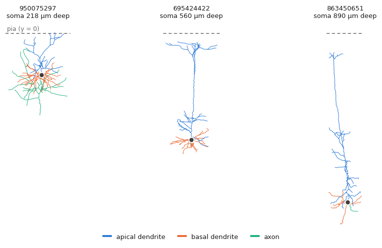
# Colour-coded, the three compartments and the reason for separating them are obvious. Note how the apical
# dendrite (blue) stretches to reach the pia while the basal bush (orange) stays put:
import matplotlib.pyplot as plt
PALETTE = {1: "#3d3d3d", 2: "#1baf7a", 3: "#eb6834", 4: "#2a78d6"}
fig, axes = plt.subplots(1, 3, figsize=(8.2, 4.6))
for ax, n in zip(axes, nl.idx[["ace-nil-mud/950075297_Manual_Upright",
"ace-new-let/695424422_Manual_Upright",
"ace-net-tug/863450651_Manual_Upright"]]):
navis.plot2d(n, method="2d", view=("x", "y"), ax=ax,
color_by=n.nodes.label.values, palette=PALETTE, lw=0.6)
ax.axhline(0, color="grey", ls="--", lw=1) # the pia
# %%
# 
#
# ## Extracting the features
#
# The call itself is a one-liner:
feats = navis.ivscc_features(nl)
feats.shape
# %%
# ```
# (25, 102)
# ```
#
# One row per neuron, 102 columns. Every column is either prefixed with the compartment it describes or is
# a whole-cell feature:
# %%
# === "Per compartment"
#
# Prefixed `axon_`, `basal_dendrite_` or `apical_dendrite_` and computed on that compartment alone.
#
# | Group | Features |
# |-------|----------|
# | Size | `num_nodes`, `total_length`, `extent_x/y/z` |
# | Topology | `num_branches`, `num_branch_points`, `num_tips`, `max_branch_order` |
# | Shape | `mean_contraction`, `bifurcation_angle_local`, `bifurcation_angle_remote` |
# | Radius | `mean_diameter`, `total_surface`, `total_volume`, `parent_daughter_ratio` |
# | Relative to soma | `bias_x`, `bias_y`, `soma_percentile_x/y`, `max_euclidean_distance`, `max_path_length`, `early_branch_path` |
# | Where it leaves | `num_stems`, `exit_distance`, `exit_theta` |
#
# === "Whole cell"
#
# No prefix - these describe the neuron rather than one of its parts.
#
# | Feature | Description |
# |---------|-------------|
# | `soma_radius` | Radius of the soma node |
# | `soma_surface` | Soma surface area, as a sphere |
# | `num_stems` | Neurites leaving the soma, across all compartments |
#
# === "Between compartments"
#
# For each **ordered pair** of compartments, how their depth distributions relate.
#
# | Feature | Description |
# |---------|-------------|
# | `_frac_above_` | Fraction of *a*'s nodes above *b*'s full depth range |
# | `_frac_intersect_` | Fraction of *a*'s nodes inside it |
# | `_frac_below_` | Fraction below it |
# | `_emd_with_` | Earth mover's distance between the two depth distributions |
#
# The three fractions partition *a*'s nodes and so sum to 1. The EMD is symmetric and therefore
# recorded once per pair, not twice.
#
# Picking one cell and a handful of columns:
feats.loc["ace-new-let/695424422_Manual_Upright",
["apical_dendrite_total_length", "apical_dendrite_num_tips",
"apical_dendrite_max_branch_order", "apical_dendrite_extent_y",
"basal_dendrite_total_length", "basal_dendrite_extent_y",
"num_stems", "soma_radius"]].round(2)
# %%
# ```
# apical_dendrite_total_length 3137.62
# apical_dendrite_num_tips 27.00
# apical_dendrite_max_branch_order 13.00
# apical_dendrite_extent_y 553.22
# basal_dendrite_total_length 1890.64
# basal_dendrite_extent_y 132.26
# num_stems 11.00
# soma_radius 6.38
# ```
#
# !!! note "Units in, units out"
# Features are reported in the neuron's own coordinate units and are never rescaled - we loaded these
# as microns, so lengths are microns, areas µm², angles degrees (except `exit_theta`, which is
# radians). Nothing is normalised, so **don't mix neurons in different units** in one call.
#
# ## The coordinate frame is not optional
#
# Before going any further: here is the thing that will silently ruin your results.
#
# !!! danger "`y` must be cortical depth"
# A good half of the IVSCC features - `bias_y`, `soma_percentile_y` and every overlap feature - are
# statements about **depth**, and they read depth off the `y` axis, with *larger `y` meaning closer to
# the pia*. {{ navis }} cannot check this for you: an unaligned neuron produces exactly the same
# columns, filled with numbers that mean nothing. Align first, then measure.
#
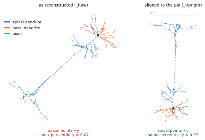
# This is why we reached for `_Upright` rather than `_Raw` earlier. The `_Raw` files make the point - same
# cells, same reconstructions, only the frame differs:
raw = navis.NeuronList([])
for bildid in CELLS:
raw += bil.get_neurons(bil.list_files(bildid, pattern="*_Raw.swc"), units="um")
# %%
# 
#
# Run those through [`ivscc_features`][navis.ivscc_features] too, and compare the averages:
feats_raw = navis.ivscc_features(raw)
cols = ["apical_dendrite_soma_percentile_y", "apical_dendrite_bias_y",
"apical_dendrite_frac_above_basal_dendrite",
"apical_dendrite_num_tips", "apical_dendrite_num_branch_points"]
pd.DataFrame({"upright": feats[cols].mean(), "raw": feats_raw[cols].mean()}).round(3)
# %%
# ```
# upright raw
# apical_dendrite_soma_percentile_y 0.970 0.066
# apical_dendrite_bias_y 482.040 -421.332
# apical_dendrite_frac_above_basal_dendrite 0.694 0.000
# apical_dendrite_num_tips 31.280 31.280
# apical_dendrite_num_branch_points 22.120 22.120
# ```
#
# In the raw frame the apical dendrite appears to sit *below* the soma (`soma_percentile_y` 0.97
# :octicons-arrow-right-24: 0.07) and `bias_y` flips sign outright - these files use image coordinates,
# where `y` grows *downwards*. Not one of those depth numbers is usable.
#
# The counts, meanwhile, are bit-identical: `num_tips` and `num_branch_points` are properties of the tree,
# not of the frame it is drawn in.
#
# ??? question "How do I get my own neurons upright?"
# If your data doesn't ship a pre-aligned variant you have to build the transform yourself - there is
# no one-size rotation. Two common routes: register to a template brain with [`navis.xform_brain`][]
# (see the [transforms tutorial](../6_misc/tutorial_misc_01_transforms)), or, if you know two points
# on the pia and white matter, construct the rotation and apply it with [`navis.xform`][]. Flipping a
# sign is enough when the axis is right but points the wrong way:
# ```python
# for n in nl:
# n.nodes["y"] *= -1
# ```
#
# ## Reading the overlap features
#
# The overlap block is the part that is specific to layered cortex, and it is easiest to understand by
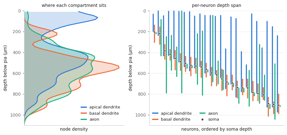
# looking at where the compartments actually sit. Pooled over all 25 cells, each compartment has its own
# depth signature - the apical piles up in the top 100 µm (the tuft), the basal hugs the somas around
# 550 µm:
# %%
# 
#
# That is exactly what the overlap features put numbers on:
ov = [c for c in feats.columns if "frac_" in c or "emd_" in c]
feats.loc["ace-new-let/695424422_Manual_Upright", ov].round(3)
# %%
# ```
# axon_frac_above_basal_dendrite 0.000
# axon_frac_intersect_basal_dendrite 1.000
# axon_frac_below_basal_dendrite 0.000
# axon_emd_with_basal_dendrite 12.611
# axon_frac_above_apical_dendrite 0.000
# axon_frac_intersect_apical_dendrite 1.000
# axon_frac_below_apical_dendrite 0.000
# axon_emd_with_apical_dendrite 283.479
# basal_dendrite_frac_above_axon 0.376
# basal_dendrite_frac_intersect_axon 0.380
# basal_dendrite_frac_below_axon 0.244
# basal_dendrite_frac_above_apical_dendrite 0.000
# basal_dendrite_frac_intersect_apical_dendrite 0.865
# basal_dendrite_frac_below_apical_dendrite 0.135
# basal_dendrite_emd_with_apical_dendrite 279.485
# apical_dendrite_frac_above_axon 0.969
# apical_dendrite_frac_intersect_axon 0.014
# apical_dendrite_frac_below_axon 0.017
# apical_dendrite_frac_above_basal_dendrite 0.858
# apical_dendrite_frac_intersect_basal_dendrite 0.142
# apical_dendrite_frac_below_basal_dendrite 0.000
# ```
#
# Read the first block as "100% of this axon lies within the depth range spanned by the basal dendrite" -
# unsurprising, given this cell's axon is a 19-node stub (see the caveats below). The apical dendrite is
# the informative one: 97% of it sits above the axon and 86% above the basal dendrite. Note that the
# relationship is *not* symmetric - only 38% of the basal dendrite sits above the axon, because the two
# are asking different questions about different reference ranges.
#
# ## Putting them to work
#
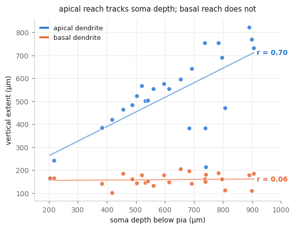
# A quick demonstration that these features carry real signal. Cortical depth is the organising variable
# in this dataset, so correlate a few features against it:
# The pia is at y = 0 and cortex runs to negative y, so depth is just -y
soma_depth = pd.Series({n.id: -n.soma_pos[0][1] for n in nl})
for col in ["apical_dendrite_extent_y", "apical_dendrite_bias_y",
"apical_dendrite_max_path_length", "basal_dendrite_extent_y"]:
print(f"{col:<34} r = {feats[col].corr(soma_depth):+.2f}")
# %%
# ```
# apical_dendrite_extent_y r = +0.70
# apical_dendrite_bias_y r = +0.66
# apical_dendrite_max_path_length r = +0.55
# basal_dendrite_extent_y r = +0.06
# ```
# %%
# 
#
# The apical dendrite scales with soma depth - it has further to climb, so it climbs further. The basal
# dendrite is flat: a compact local bush of much the same size wherever the soma sits. Splitting the
# compartments is what makes that visible; measured as one tree the two effects would partly cancel.
#
# !!! warning "n = 25"
# This is a demo, not a result - two dozen cells from mixed Cre lines. Treat the numbers as an
# illustration of what the features respond to.
#
# ## Adding your own features
#
# The feature set is just a list of classes, so you can extend it. Subclass `CompartmentFeatures` to get
# a compartment handed to you already subset out, record whatever you like, and pass it via `features`:
from navis.morpho.ivscc import CompartmentFeatures
class ApicalTuftFeatures(CompartmentFeatures):
"""Fraction of the apical dendrite sitting in the top 200 µm of cortex."""
compartment = "apical_dendrite"
def extract_features(self):
y = self.neuron.nodes.y.values # `self.neuron` is just the apical dendrite
self.record_feature("frac_in_tuft", float((y > -200).mean()))
return self.features
tuft = navis.ivscc_features(nl, features=[ApicalTuftFeatures])
print("correlation with soma depth: %+.2f"
% tuft.apical_dendrite_frac_in_tuft.corr(soma_depth))
# %%
# ```
# correlation with soma depth: -0.90
# ```
#
# ??? info "What you get inside a feature class"
# | Attribute | What it is |
# |-----------|------------|
# | `self.neuron` | the compartment, already subset out (the full neuron for non-compartment classes) |
# | `self.ctx.neuron` | the **whole** neuron, rooted at its soma |
# | `self.ctx.dist_to_root` | geodesic distance from every node to the soma, computed once and shared |
# | `self.soma`, `self.soma_pos`, `self.soma_radius` | soma node ID, position and radius |
# | `self.record_feature(name, value)` | records a feature, prefixing it with the compartment name |
#
# Call `super().extract_features()` first if you want the standard features *plus* yours, and note
# that `features=` replaces the default list - pass `DEFAULT_FEATURES + [MyFeatures]` to add to it.
#
# ## Caveats
#
# Two things worth knowing before you trust a column.
#
# !!! warning "Patch-seq axons are cut off"
# A slice is 300 µm thick and axons leave it. In this set the axons run from 13 µm to 3.7 mm of cable
# and **12 of the 25** cells have an axon with no branch point at all - so their
# `axon_bifurcation_angle_*` are `NaN` and their `axon_total_length` says more about the slice than
# about the cell. Dendrite features are largely fine; axon features from slice data are not
# comparable across cells.
#
# Not every cell has every compartment - interneurons have no apical dendrite, and a reconstruction may
# simply not include the axon. `missing_compartments` decides what happens then:
#
# | Value | Behavior |
# |-------|----------|
# | `"ignore"` (default) | Skip that compartment. Its columns are `NaN` for that neuron |
# | `"skip"` | Drop the neuron from the result entirely |
# | `"raise"` | Raise a `CompartmentNotFoundError` |
#
# The same applies to a neuron with no `label` column at all - it counts as "no compartments found"
# rather than an error, so a mixed batch won't blow up on you.
#
# ## Where next
#
# - [IVSCC on EM data](zzz_tutorial_morpho_06_ivscc_em) - getting MICrONS reconstructions into a state
# where these features mean something
# - [Analyze morphology](tutorial_morpho_01_analyze) - the general-purpose morphometrics, for neurons that
# aren't cortical
# - [Label propagation](tutorial_morpho_02_label_prop) and
# [axon-dendrite splits](tutorial_morpho_03_ad_split) - ways to *get* compartment labels when your data
# doesn't come with them
# - [Cortical neurons](../1e_plotting_examples/tutorial_plotting_ex_00_cortex) - plotting this kind of data,
# arranged by soma depth
# - [NBLAST](../5_nblast/tutorial_nblast_00_intro) - comparing neurons by shape rather than by feature vector
# %%
# *[IVSCC]: In Vitro Single Cell Characterization - the Allen Institute's pipeline for profiling cortical neurons.
# *[SWC]: A plain-text format storing a neuron skeleton as a table of connected nodes.
# *[Patch-seq]: Recording a cell electrophysiologically, then extracting its contents for sequencing and staining it for morphology.
# *[EM]: Electron Microscopy.
# *[EMD]: Earth mover's distance - the cost of turning one distribution into another.
# *[BIL]: Brain Image Library.
# mkdocs_gallery_thumbnail_path = '_static/ivscc_tut/00_thumbnail.png'