"""
Neuron Types
============
This tutorial will show you the different neuron types and how to work with them.
Depending your data/workflows, you will use different representations of neurons.
If, for example, you work with light-level data you might end up extracting point
clouds or neuron skeletons from image stacks. If, on the other hand, you work with
segmented EM data, you will typically work with meshes.
To cater for these different representations, neurons in {{ navis }} come in four flavours:
| Neuron type | Description | Core data |
|-------------------------|-----------------------------------------------------------------------|-------------------------------------|
| [`navis.TreeNeuron`][] | A hierarchical skeleton consisting
of nodes and edges. | - `.nodes`: the SWC node table |
| [`navis.MeshNeuron`][] | A mesh with faces and vertices. | - `.vertices`: `(N, 3)` array of x/y/z vertex coordinates
- `.faces`: `(M, 3)` array of faces |
| [`navis.VoxelNeuron`][] | An image represented by either a
2d array of voxels or a 3d voxel grid. | - `.voxels`: `(N, 3)` array of voxels
- `.values`: `(N, )` array of values (i.e. intensity)
- `.grid`: `(N, M, K)` 3D voxelgrid |
| [`navis.Dotprops`][] | A cloud of points, each with an
associated local vector. | - `.points`: `(N, 3)` array of point coordinates
- `.vect`: `(N, 3)` array of normalized vectors |
Note that functions in {{ navis }} may only work on a subset of neuron types:
check out this [table](../../api.md#neuron-types-and-functions) in the [API](../../api.md)
reference for details. If necessary, {{ navis }} can help you convert between the
different neuron types (see further [below](#converting-neuron-types))!
!!! important
In this guide we introduce the different neuron types using data bundled with {{ navis }}.
To learn how to load your own neurons into {{ navis }} please see the tutorials on
[Import/Export](../../gallery#import-export).
## TreeNeurons
[`TreeNeurons`][navis.TreeNeuron] represent a neuron as a tree-like "skeleton" - effectively a directed
acyclic graph, i.e. they consist of nodes and each node connects to at most one parent.
This format is commonly used to describe a neuron's topology and often shared using
[SWC](http://www.neuronland.org/NLMorphologyConverter/MorphologyFormats/SWC/Spec.html) files.
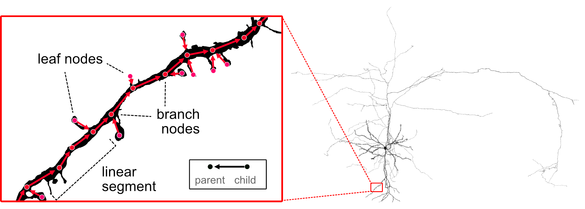
A [`navis.TreeNeuron`][] is typically loaded from an SWC file via [`navis.read_swc`][]
but you can also constructed one yourself from e.g. `pandas.DataFrame` or a `networkx.DiGraph`.
See the [skeleton I/O](../0_io/tutorial_io_00_skeletons) tutorial for details.
{{ navis }} ships with a couple example *Drosophila* neurons from the Janelia hemibrain project published
in [Scheffer et al. (2020)](https://elifesciences.org/articles/57443) and available at
(see also the [neuPrint tutorial](../4_remote/tutorial_remote_00_neuprint)):
"""
# %%
import navis
# Load one of the example neurons
sk = navis.example_neurons(n=1, kind="skeleton")
# Inspect the neuron
sk
# %%
# [`navis.TreeNeuron`][] stores nodes and other data as attached `pandas.DataFrames`:
# %%
sk.nodes.head()
# %%
# ## MeshNeurons
#
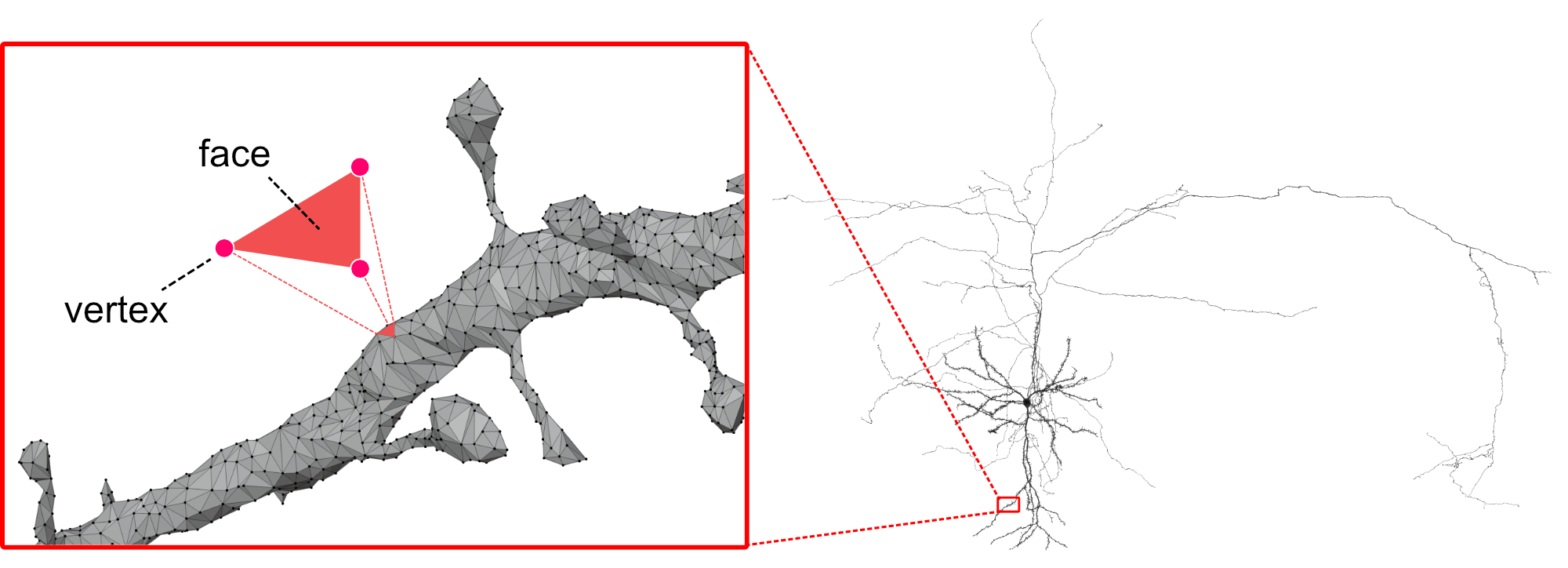
# [`MeshNeurons`][navis.MeshNeuron] consist of vertices and faces, and are a typical output of e.g. image segmentation.
#
# 
#
# A [`navis.MeshNeuron`][] can be constructed from any object that has `.vertices` and `.faces` properties, a
# dictionary of `vertices` and `faces` or a file that can be parsed by `trimesh.load`.
# See the [mesh I/O](../0_io/tutorial_io_01_meshes) tutorial for details.
#
# Each of the example neurons in {{ navis }} also comes as mesh representation:
# %%
m = navis.example_neurons(n=1, kind="mesh")
m
# %%
# [`navis.MeshNeuron`][] stores vertices and faces as attached numpy arrays:
# %%
m.vertices, m.faces
# %%
# ## Dotprops
#
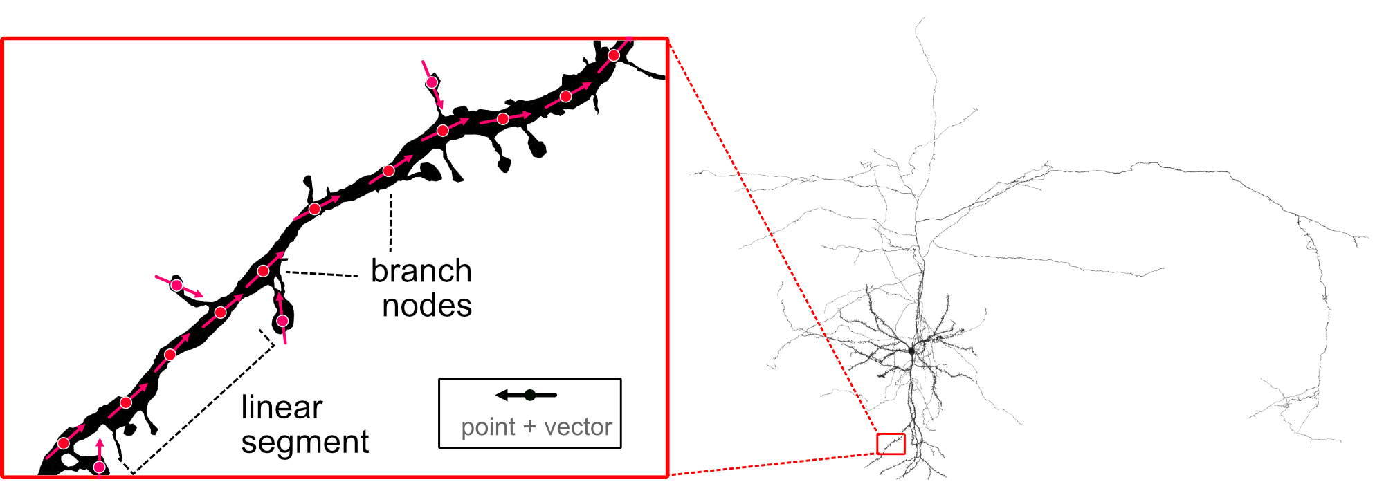
# [`Dotprops`][navis.Dotprops] represent neurons as point clouds where each point is associated with a vector
# describing the local orientation. This simple representation often comes from e.g. light-level data
# or as direvative of skeletons/meshes (see [`navis.make_dotprops`][]).
#
# 
#
# Dotprops are used e.g. for [NBLAST](../5_nblast/tutorial_nblast_00_intro). See the [dotprops I/O](../0_io/tutorial_io_02_dotprops)
# tutorial for details.
#
# [`navis.Dotprops`][] consist of `.points` and associated `.vect` (vectors). They are typically
# created from other types of neurons using [`navis.make_dotprops`][]:
# %%
# Turn our above skeleton into dotprops
dp = navis.make_dotprops(sk, k=5)
dp
# %%
dp.points, dp.vect
# %%
# Check out the NBLAST tutorial for further details on dotprops!
#
# ## VoxelNeurons
#
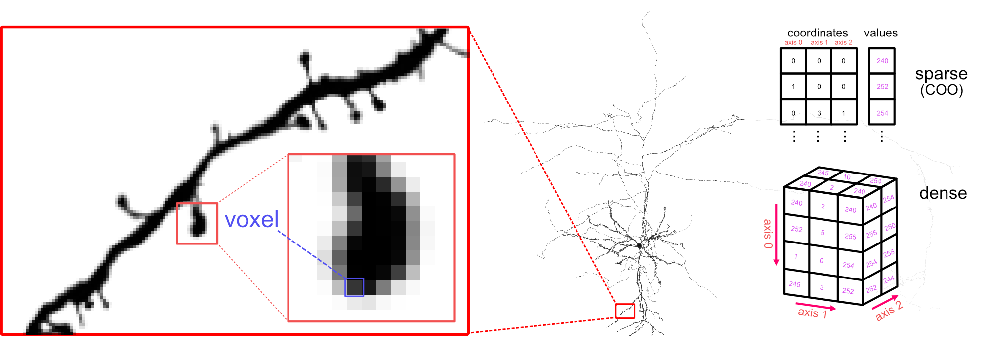
# [`VoxelNeurons`][navis.VoxelNeuron] represent neurons as either 3d image or x/y/z voxel coordinates
# typically obtained from e.g. light-level microscopy.
#
# 
#
# [`navis.VoxelNeuron`][] consist of either a dense 3d `(N, M, K)` array (a "grid") or a sparse 2d `(N, 3)`
# array of voxel coordinates (COO format). You will probably find yourself loading these
# data from image files (e.g. `.nrrd` via [`navis.read_nrrd()`][navis.read_nrrd]). That said we can
# also "voxelize" other neuron types to produce [`VoxelNeurons`][navis.VoxelNeuron]:
# Load an example mesh
m = navis.example_neurons(n=1, kind="mesh")
# Voxelize:
# - with a 0.5 micron voxel size
# - some Gaussian smoothing
# - use number of vertices (counts) for voxel values
vx = navis.voxelize(m, pitch="0.5 microns", smooth=2, counts=True)
vx
# %%
# This is the grid representation of the neuron:
vx.grid.shape
# %%
# And this is the `(N, 3)` voxel coordinates + `(N, )` values sparse representation of the neuron:
vx.voxels.shape, vx.values.shape
# %%
# !!! note
#
# You may have noticed that all neurons share some properties irrespective of their type,
# for example `.id`, `.name` or `.units`. These properties are optional and can
# be set when you first create the neuron, or at a later point.
#
# In particular the `.id` property is important because many functions in {{ navis }}
# will return results that are indexed by the neurons' IDs. If `.id` is not set
# explicitly, it will default to some rather cryptic random UUID - you have been warned!
# :wink:
#
# ## Neuron meta data
#
# ### Connectors
#
# {{ navis }} was designed with connectivity data in mind! Therefore, each neuron - regardless of
# type - _can_ have a `.connectors` table. Connectors are meant to bundle all kinds of connections:
# pre- & postsynapses, electrical synapses, gap junctions and so on.
#
# A connector table must minimally contain an `x/y/z` coordinate and a `type` for each connector.
# Here is an example of a connector table:
# %%
n = navis.example_neurons(1)
n.connectors.head()
# %%
# Connector tables aren't just passive meta data: certain functions in {{ navis }} use or even
# require them. The most obvious example is probably for plotting:
# Plot neuron including its connectors
fig, ax = navis.plot2d(
n, # the neuron
connectors=True, # plot the neurons' connectors
color="k", # make the neuron black
cn_size=3, # slightly increase connector size
view=("x", "-z"), # set frontal view
method="2d" # connectors are better visible in 2d
)
# %%
# In above plot, red dots are presynapses (outputs) and cyan dots are postsynapses (inputs).
#
# ### Somas
#
# Unless a neuron is truncated, it should have a soma somewhere. Knowing where the soma is can
# be very useful, e.g. as point of reference for distance calculations or for plotting.
# Therefore, {{ navis }} neurons have a `.soma` property:
# %%
n = navis.example_neurons(1)
n.soma
# %%
# In case of this exemplary [`navis.TreeNeuron`][], the `.soma` points to an ID in the node table.
# We can also get the position:
# %%
n.soma_pos
# %%
# Other neuron types also support soma annotations but they may look slightly different. For a
# [`navis.MeshNeuron`][], annotating a node position makes little sense. Instead, we track
# the x/y/z position directly:
# %%
m = navis.example_neurons(1, kind="mesh")
m.soma_pos
# %%
# For the record: `.soma` / `.soma_pos` can be set manually like any other property (there are
# some checks and balances to avoid issues) and can also be `None`:
# Set the skeleton's soma on node with ID 1
n.soma = 1
n.soma
# %%
# Drop soma from MeshNeuron
m.soma_pos = None
# %%
# ### Units
#
# {{ navis }} supports assigning units to neurons. The neurons shipping with {{ navis }}, for example, are in 8x8x8nm voxel space[^1]:
#
# [^1]: The example neurons are from the [Janelia hemibrain connectome](https://www.janelia.org/project-team/flyem/hemibrain) project which as imaged at 8x8x8nm resolution.
# %%
m = navis.example_neurons(1, kind="mesh")
print(m.units)
# %%
# To set the neuron's units simply use a descriptive string:
# %%
m.units = "10 micrometers"
print(m.units)
# %%
# !!! note
# Setting the units as we did above does not actually change the neuron's coordinates. It
# merely sets a property that can be used by other functions to interpret the neuron's
# coordinate space. See below on how to convert the units of a neuron.
#
# Tracking units is good practice in general but is also very useful in a variety of scenarios:
#
# First, certain {{ navis }} functions let you pass quantities as unit strings:
# Load example neuron which is in 8x8x8nm space
n = navis.example_neurons(1, kind="skeleton")
# Resample to 1 micrometer
rs = navis.resample_skeleton(n, resample_to="1 um")
# %%
# Second, {{ navis }} optionally uses the neuron's units to make certain properties more
# interpretable. By default, properties like cable length or volume are returned in the
# neuron's units, i.e. in 8x8x8nm voxel space in our case:
print(n.cable_length)
# %%
# You can tell {{ navis}} to use the neuron's `.units` to make these properties more readable:
navis.config.add_units = True
print(n.cable_length)
navis.config.add_units = False # reset to default
# %%
# !!! note
# Note that `n.cable_length` is now a `pint.Quantity` object. This may make certain operations
# a bit more cumbersome which is why this feature is optional. You can to a float by calling
# `.magnitude`:
#
# ```python
# n.cable_length.magnitude
# ```
# %%
# Check out Pint's [documentation](https://pint.readthedocs.io/en/stable/) to learn more.
#
# To actually convert the neuron's coordinate space, you have two options:
#
# === "Multiply/Divide"
#
# You can multiply or divide any neuron or [`NeuronList`][navis.NeuronList] by a number
# to change the units:
#
# ```python
# # Example neuron are in 8x8x8nm voxel space
# n = navis.example_neurons(1)
# # Multiply by 8 to get to nanometer space
# n_nm = n * 8
# # Divide by 1000 to get micrometers
# n_um = n_nm / 1000
# ```
#
# For non-isometric conversions you can pass a vector of scaling factors:
# ```python
# neuron * [4, 4, 40]
# ```
# Note that for `TreeNeurons`, this is expected to be scaling factors for
# `(x, y, z, radius)`.
#
#
# === "Convert units"
#
# If your neuron has known units, you can let {{ navis }} do the conversion for you:
#
# ```python
# n = navis.example_neurons(1)
# # Convert to micrometers
# n_um = n.convert_units("micrometers")
# ```
#
# !!! experiment "Addition & Subtraction"
# Multiplication and division will scale the neuro as you've seen above.
# Similarly, adding or subtracting to/from neurons will offset the neuron's coordinates:
# ```python
# n = navis.example_neurons(1)
#
# # Convert to microns
# n_um = n.convert_units("micrometers")
#
# # Add 100 micrometers along all axes to the neuron
# n_offset = n + 100
#
# # Subtract 100 micrometers along just one axis
# n_offset = n - [0, 0, 100]#
# ```
#
# ## Operating on neurons
#
# Above we've already seen examples of passing neurons to functions - for example [`navis.plot2d(n)`][navis.plot2d].
#
# For some {{ navis }} functions, neurons offer have shortcut "methods":
# %% [markdown]
# === "Using shorthand methods"
# ```python
# import navis
# sk = navis.example_neurons(1, kind='skeleton')
#
# sk.reroot(sk.soma, inplace=True) # reroot the neuron to its soma
#
# lh = navis.example_volume('LH')
# sk.prune_by_volume(lh, inplace=True) # prune the neuron to a volume#
#
# sk.plot3d(color='red') # plot the neuron in 3d
# ```
#
# === "Using NAVis functions"
# ```python
# import navis
# sk = navis.example_neurons(1, kind='skeleton')
#
# navis.reroot_skeleton(sk, sk.soma, inplace=True) # reroot the neuron to its soma
#
# lh = navis.example_volume('LH')
# navis.in_volume(sk, lh, inplace=True) # prune the neuron to a volume
#
# navis.plot3d(sk, color='red') # plot the neuron in 3d
# ```
#
# !!! note
#
# In some cases the shorthand methods might offer only a subset of the full function's functionality.
#
# ### The `inplace` parameter
#
# The `inplace` parameter is part of many {{ navis }} functions and works like e.g. in the `pandas` library:
#
# - if `#!python inplace=True` operations are performed directly on the input neuron(s)
# - if `#!python inplace=False` (default) a modified copy of the input is returned and the input is left unchanged
#
# If you know you don't need the original, you can use `#!python inplace=True` to save memory (and a bit of time):
# %%
# Load a neuron
n = navis.example_neurons(1)
# Load an example neuropil
lh = navis.example_volume("LH")
# Prune neuron to neuropil but leave original intact
n_lh = n.prune_by_volume(lh, inplace=False)
print(f"{n.n_nodes} nodes before and {n_lh.n_nodes} nodes after pruning")
# %%
# ## All neurons are equal...
#
# ... but some are more equal than others.
#
# In Python the `==` operator compares two objects:
# %%
1 == 1
# %%
2 == 1
# %%
# For {{ navis }} neurons this is comparison done by looking at the neurons' attribues:
# morphologies (soma & root nodes, cable length, etc) and meta data (name).
# %%
n1, n2 = navis.example_neurons(n=2)
n1 == n1
# %%
n1 == n2
# %%
# To find out which attributes are compared, check out the neuron's `.EQ_ATTRIBUTES` property:
# %%
navis.TreeNeuron.EQ_ATTRIBUTES
# %%
# Edit this list to establish your own criteria for equality.
#
# ## Making custom changes
#
# Under the hood {{ navis }} calculates certain properties when you load a neuron: e.g. it produces
# a graph representation (`.graph` or `.igraph`) and a list of linear segments (`.segments`) for
# [`TreeNeurons`][navis.TreeNeuron]. These data are attached to a neuron and are crucial for many
# functions. Therefore {{ navis }} makes sure that any changes to a neuron automatically propagate
# into these derived properties. See this example:
# %%
n = navis.example_neurons(1, kind="skeleton")
print(f"Nodes in node table: {n.nodes.shape[0]}")
print(f"Nodes in graph: {len(n.graph.nodes)}")
# %%
# Making changes will cause the graph representation to be regenerated:
# %%
n.prune_by_strahler(1, inplace=True)
print(f"Nodes in node table: {n.nodes.shape[0]}")
print(f"Nodes in graph: {len(n.graph.nodes)}")
# %%
# If, however, you make changes to the neurons that do not use built-in functions there is a chance that
# {{ navis }} won't realize that things have changed and properties need to be regenerated!
# %%
n = navis.example_neurons(1)
print(f"Nodes in node table before: {n.nodes.shape[0]}")
print(f"Nodes in graph before: {len(n.graph.nodes)}")
# Truncate the node table by 55 nodes
n.nodes = n.nodes.iloc[:-55].copy()
print(f"\nNodes in node table after: {n.nodes.shape[0]}")
print(f"Nodes in graph after: {len(n.graph.nodes)}")
# %%
# Here, the changes to the node table automatically triggered a regeneration of the graph. This works
# because {{ navis }} checks hash values of neurons and in this instance it detected that the node
# node table - which represents the core data for [`TreeNeurons`][navis.TreeNeuron] - had changed.
# It would not work the other way around: changing the graph does not trigger changes in the node table.
#
# Again: as long as you are using built-in functions, you don't have to worry about this. If you do
# run some custom manipulation of neurons be aware that you might want to make sure that the data
# structure remains intact. If you ever need to manually trigger a regeneration you can do so like this:
# %%
# Clear temporary attributes of the neuron
# ```python
# n._clear_temp_attr()
# ```
# %%
# ## Converting neuron types
#
# {{ navis }} provides a couple functions to move between neuron types:
#
# - [`navis.make_dotprops`][]: Convert any neuron to dotprops
# - [`navis.skeletonize`][]: Convert any neuron to a skeleton
# - [`navis.mesh`][]: Convert any neuron to a mesh
# - [`navis.voxelize`][]: Convert any neuron to a voxel grid
#
# In particular meshing and skeletonizing are non-trivial and you might have to play around with the
# parameters to optimize results with your data! Let's demonstrate on some example:
# %%
# Start with a mesh neuron
m = navis.example_neurons(1, kind="mesh")
# Skeletonize the mesh
s = navis.skeletonize(m)
# Make dotprops (this works from any other neuron type
dp = navis.make_dotprops(s, k=5)
# Voxelize the mesh
vx = navis.voxelize(m, pitch="2 microns", smooth=1, counts=True)
# Mesh the voxels
mm = navis.mesh(vx.threshold(0.5))
# %%
# Inspect the results:
# Co-visualize the mesh and the skeleton
navis.plot3d(
[m, s],
color=[(0.7, 0.7, 0.7, 0.2), "r"], # transparent mesh, skeleton in red
radius=False, # False so that skeleton is drawn as a line
)
# %%
# Co-visualize the mesh and the dotprops
navis.plot3d(
[m, dp],
color=[(0.7, 0.7, 0.7, 0.2), "r"], # transparent mesh, dotprops in red
)
# %%
# Co-visualize the mesh and the dotprops
# (note that plotly is not great at visualizing voxels)
navis.plot3d([m * 8, vx])
# %%
# Co-visualize the original mesh and the meshed voxels
navis.plot3d([vx, mm], fig_autosize=True)
# %%
# ## Neuron attributes
#
# This is a *selection* of neuron class (i.e. [`navis.TreeNeuron`][], [`navis.MeshNeuron`][], etc.) attributes.
#
# All neurons have this:
#
# - `name`: a name
# - `id`: a (hopefully unique) identifier - defaults to random UUID if not set explicitly
# - `bbox`: Bounding box of neuron
# - `units` (optional): spatial units (e.g. "1 micrometer" or "8 nanometer" voxels)
# - `connectors` (optional): connector table
#
# Only for [`TreeNeurons`][navis.TreeNeuron]:
#
# - `nodes`: node table
# - `cable_length`: cable length(s)
# - `soma`: node ID(s) of soma (if applicable)
# - `root`: root node ID(s)
# - `segments`: list of linear segments
# - `graph`: NetworkX graph representation of the neuron
# - `igraph`: iGraph representation of the neuron (if library available)
#
# Only for [`MeshNeurons`][navis.MeshNeuron]:
#
# - `vertices`/`faces`: vertices and faces
# - `volume`: volume of mesh
# - `soma_pos`: x/y/z position of soma
#
# Only for [`VoxelNeurons`][navis.VoxelNeuron]:
#
# - `voxels`: `(N, 3)` sparse representation
# - `grid`: `(N, M, K)` voxel grid representation
#
# Only for [`Dotprops`][navis.Dotprops]:
#
# - `points` `(N, 3`) x/y/z points
# - `vect`: `(N, 3)` array of the vector associated with each point
#
# All above attributes can be accessed via [`NeuronLists`][navis.NeuronList] containing the neurons. In addition you can also get:
#
# - `is_mixed`: returns `True` if list contains more than one neuron type
# - `is_degenerated`: returns `True` if list contains neurons with non-unique IDs
# - `types`: tuple with all types of neurons in the list
# - `shape`: size of neuronlist `(N, )`
#
# All attributes and methods are accessible through auto-completion.
#
# ## What next?
#
#
#
# - :material-cube:{ .lg .middle } __Lists of Neurons__
#
# ---
#
# Check out the guide on lists of neurons.
#
# [:octicons-arrow-right-24: NeuronLists tutorial](../tutorial_basic_02_neuronlists)
#
# - :octicons-file-directory-symlink-16:{ .lg .middle } __Neuron I/O__
#
# ---
#
# Learn about how to load your own neurons into {{ navis }}.
#
# [:octicons-arrow-right-24: I/O Tutorials](../../gallery#import-export)
#
#