"""
Neuron Collages
===============
<!-- difficulty: intermediate -->

Arrange hundreds of neurons on a single page.

!!! important "This example is not executed"
    Like the [light-level skeletonization tutorial](../0_io/zzz_tutorial_io_05_skeletonize), this one is
    *not* run when the documentation is built - it pulls 200 skeletons from a live neuPrint server, which
    is slow and needs a token. The code is real and runnable; the outputs and figures shown here are
    statically embedded.

Sooner or later you will want to put *a lot* of neurons on one page: a plate showing every cell type in a
region, a poster, a supplementary "here is the whole dataset" figure. Doing that by hand - one subplot per
neuron, then fiddling with the limits until the sizes look right - is tedious, and a regular grid spends
most of the paper on the empty space around each arbor.

[`navis.plot_collage`][] does the arranging for you: it scales and moves *copies* of your neurons onto a
page and plots them. The originals are left untouched.

```mermaid
graph LR
    A[NeuronList] --> B{layout};
    B -->|"grid"| C[one neuron<br>per cell];
    B -->|"dense"| D[packed by<br>bounding box];
    D -->|"occupancy=True"| E[packed by<br>the arbors themselves];
```

| Layout | What it does | Reach for it when |
|--------|--------------|-------------------|
| `"grid"` | one neuron per cell of a regular grid | you want to *read* individual neurons - a catalogue |
| `"dense"` | packs them as tightly as they will go, keeping their relative sizes | you want the page *full* - a plate or a poster |

"""

# %%
# ## The neurons
#
# We will use the central complex of the male CNS dataset on [neuPrint](https://neuprint.janelia.org).
# See the [neuPrint tutorial](../4_remote/tutorial_remote_00_neuprint) for how to set up the client and
# where to get a token.

import navis
import navis.interfaces.neuprint as neu

client = neu.Client("https://neuprint.janelia.org", "male-cns:v1.0")

# Metadata for every CX neuron
meta = neu.fetch_neurons(neu.NeuronCriteria(class_="CX"), omit_rois=True)

# One neuron per cell type, 200 of them
nl = neu.fetch_skeletons(
    meta.drop_duplicates("type").sample(200, random_state=42).bodyId.values
)
nl

# %%
# ```
# <class 'navis.core.neuronlist.NeuronList'> containing 200 neurons (12.3MiB)
#                type            name     id  ...   cable_length soma        units
# 0    navis.Skeleton          FB2L_L  17749  ...  224793.843750    1  8 nanometer
# 1    navis.Skeleton  P6-8P9(PB14)_L  94391  ...   81555.570312    2  8 nanometer
# ..              ...             ...    ...  ...            ...  ...          ...
# 198  navis.Skeleton        FB4A_a_L  92683  ...  192589.781250    4  8 nanometer
# 199  navis.Skeleton          ExR8_L  15458  ...  253509.984375    2  8 nanometer
# ```
#
# ## Layout 1: the grid
#
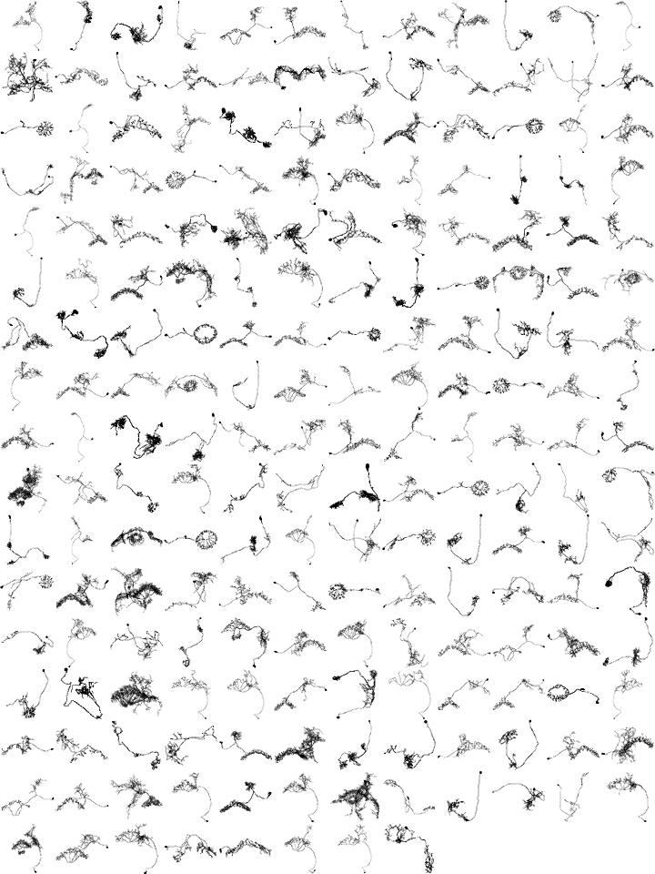
# The default. One neuron per cell, scaled to fill it:

fig, ax, placed = navis.plot_collage(nl, page_size=(6, 8), radius="lw", color="k")

# %%
# ![grid](../../../_static/collage_tut/01_grid.png)
#
# Two arguments there are worth a word before we go on:
#
# !!! tip "`page_size` and `radius`"
#     **`page_size`** is the figure size in inches and defaults to A4 - which, at the default `dpi=300`,
#     is a 2481 × 3507 pixel figure. That is the right call for something you intend to print, but it
#     makes for unwieldy plots on screen, so everything here uses a smaller `(6, 8)` page.
#
#     **`radius="lw"`** maps each node's radius onto the line width instead of outlining a tube. On a page
#     with this much cable on it that reads *much* better than flat lines, for a fraction of the file size
#     of `radius=True` - see the [skeleton plotting tutorial](../1b_plotting_2d/tutorial_plotting_2d_00_skeletons).
#
# The grid takes five arguments:
#
# | Parameter | Default | Effect |
# |-----------|---------|--------|
# | `cols` | `None` | Number of columns. `None` picks whatever makes the cells as square as possible. |
# | `margin` | `0.05` | Fraction of each cell left free around the neuron. |
# | `uniform_scale` | `False` | Scale all neurons by the same factor instead of fitting each to its cell. |
# | `sort` | `False` | Sort by size, largest first. |
# | `drop_dangling` | `False` | Drop neurons off the end until the last row is full. |
#
# ### Keeping relative sizes
#
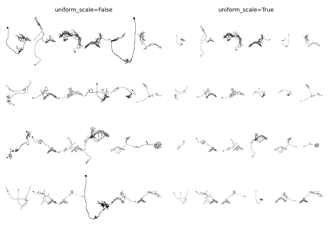
# By default each neuron is blown up until it fills its cell, so a small neuron and a large one end up
# looking the same size. `uniform_scale=True` scales all of them by the same factor instead - the two
# side by side:

sub = nl.sample(24, random_state=1)

navis.plot_collage(sub, cols=6, uniform_scale=True, page_size=(4.5, 6), radius="lw", color="k")

# %%
# ![uniform scale](../../../_static/collage_tut/02_uniform_scale.png)
#
# !!! warning "`radius` and `uniform_scale` go together"
#     Scaling a neuron scales its radii too. With the default `uniform_scale=False` every neuron gets its
#     own factor, so the line widths on the page are **not** comparable between cells - a thin neurite in a
#     small neuron can end up thicker than a thick one in a large neuron. If you plot with `radius` and want
#     the widths to mean something, use `uniform_scale=True`.
#
# ### Filling the grid
#
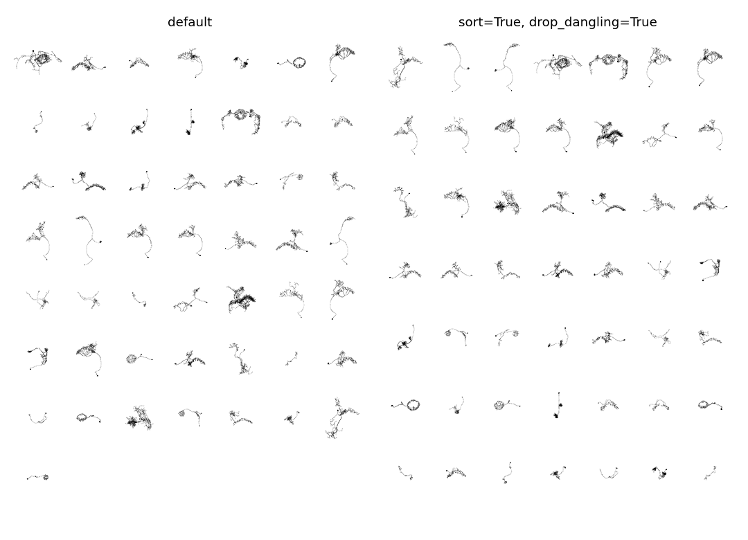
# 50 neurons into 7 columns leaves one lonely neuron on the last row (left, below). `sort=True` orders
# them by size and `drop_dangling=True` drops as many off the end as it takes to fill the grid exactly -
# together, that means the ones dropped are the smallest (right):

sub50 = nl.sample(50, random_state=2)

navis.plot_collage(
    sub50,
    cols=7,
    uniform_scale=True,
    sort=True,
    drop_dangling=True,
    page_size=(4.5, 6),
    radius="lw",
    color="k",
)

# %%
# ```
# INFO  : Dropping 1 neuron(s) to fill the grid: 49 of 50 plotted.
# ```
#
# ![sort](../../../_static/collage_tut/03_sort.png)
#
# ## Layout 2: dense
#
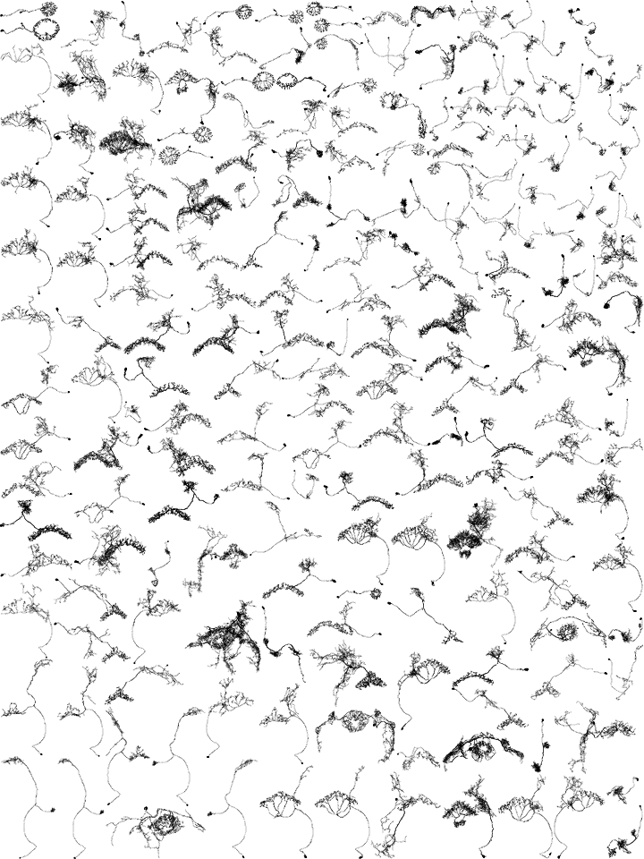
# A grid gives every neuron the same amount of paper whether it needs it or not. `layout="dense"` instead
# packs the neurons as tightly as they will go, at one common scale - so their relative sizes survive:

fig, ax, placed = navis.plot_collage(
    nl, layout="dense", page_size=(6, 8), radius="lw", color="k"
)

# %%
# ![dense](../../../_static/collage_tut/04_dense_boxes.png)
#
# ??? info "How the scale is found"
#     There is no way to compute the largest scale that still fits - so {{ navis }} searches for it. It
#     packs the neurons at some scale, asks whether they fit, and bisects: too big, halve it; fits, try
#     bigger. `iterations` (default `18`) is how many of those steps it takes, and the last one that fit is
#     the page you get. The packing itself is done by
#     [`navis-fastcore`](https://github.com/schlegelp/fastcore-rs).
#
# ### Packing the arbors instead of the boxes
#
# Look at the page above and you will notice it is not really *dense*: the packing is done on each neuron's
# **bounding box**, and a neuron fills very little of its own box. Everything inside that box is reserved
# for one neuron, empty or not.
#
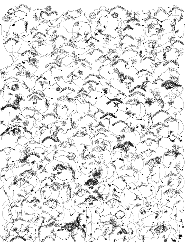
# `occupancy=True` packs the rasterised arbors instead. A neuron may then reach into another's empty space -
# even into the loop of another neuron - as long as no cable actually collides:

fig, ax, placed = navis.plot_collage(
    nl, layout="dense", occupancy=True, page_size=(6, 8), radius="lw", color="k"
)

# %%
# === "occupancy=True"
#     ![occupancy](../../../_static/collage_tut/05_dense_occupancy.png)
#
# === "occupancy=False (default)"
#     ![boxes](../../../_static/collage_tut/04_dense_boxes.png)
#
# Same 200 neurons, same page: packing the arbors draws each of them **1.37× larger** than packing their
# boxes did - close to twice the area per neuron.
#
# !!! note "It can only improve on the boxes"
#     The box packing runs first either way and hands its scale to the occupancy search as a starting
#     point, so `occupancy=True` never does *worse* than `occupancy=False` - it just costs more time.
#     Turn `occupancy_res` (default `100` px per page unit) up for a more precise fit, down for a faster one.
#
# ### Padding and rotation
#
# | Parameter | Default | Effect |
# |-----------|---------|--------|
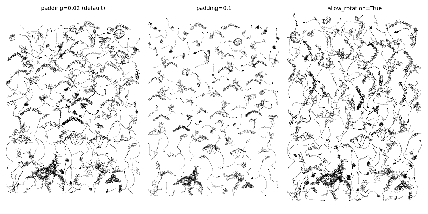
# | `padding` | `0.02` | Gap kept between neurons, in page units. Raise it to let the page breathe, lower it to squeeze. |
# | `allow_rotation` | `False` | Let neurons be turned by 90° if that packs tighter. |
#
# On 60 of our neurons, `padding=0.1` costs ~24% of the scale and `allow_rotation=True` buys back ~7%
# (default, padding and rotation, left to right below):

sub60 = nl.sample(60, random_state=3)

navis.plot_collage(
    sub60,
    layout="dense",
    occupancy=True,
    allow_rotation=True,  # or: padding=0.1
    page_size=(3.6, 5),
    radius="lw",
    color="k",
)

# %%
# ![padding and rotation](../../../_static/collage_tut/06_padding_rotation.png)
#
# ### Filling the gaps: `backfill`
#
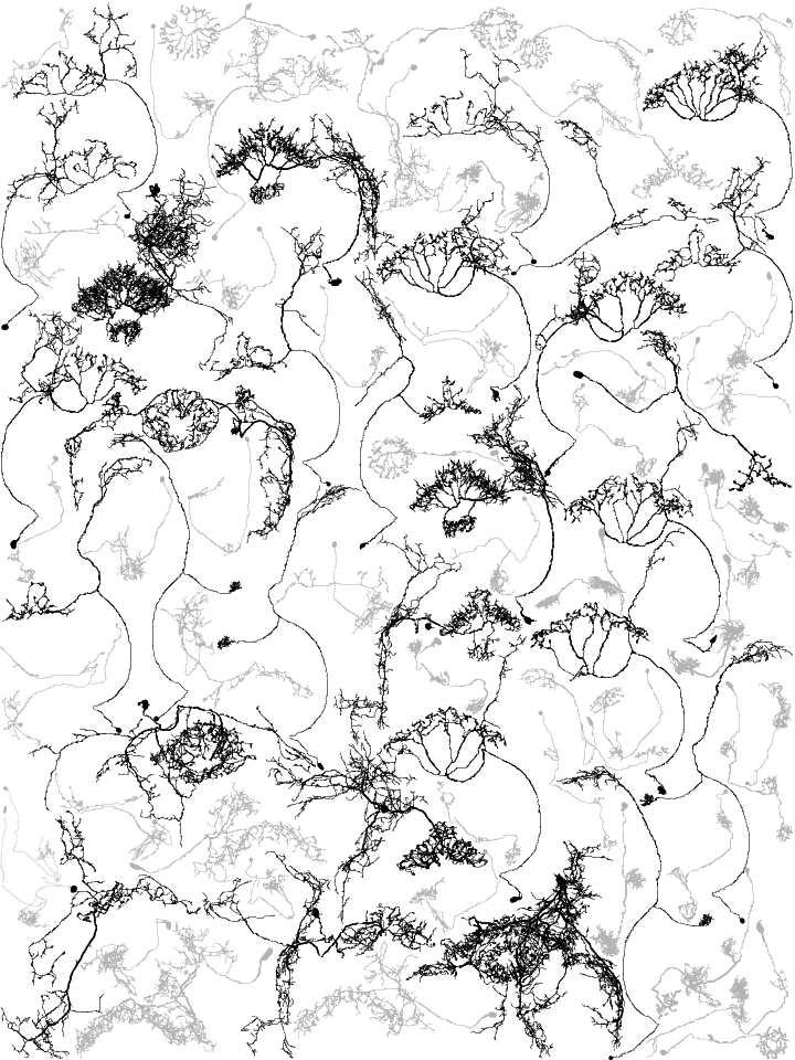
# Even packed by occupancy there are holes left, and often you have neurons you would *like* to show but
# do not need to. That is what `backfill` is for: those neurons are packed into whatever room is left over
# once `x` is placed. They do not influence the scale, and any that find no gap are silently dropped.
#
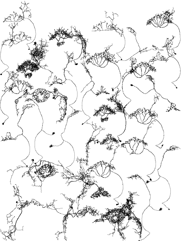
# Here the 30 largest neurons carry the page (black) and the remaining 170 are offered as backfill (grey):

import numpy as np

# Order by bounding box area in the plane we are plotting
bbox = np.array([n.bbox for n in nl])
by_size = nl[np.argsort(-np.prod(bbox[:, :2, 1] - bbox[:, :2, 0], axis=1))]

main, rest = by_size[:30], by_size[30:]

fig, ax, placed = navis.plot_collage(
    main,
    layout="dense",
    backfill=rest,
    occupancy=True,
    page_size=(6, 8),
    radius="lw",
    color=["k"] * len(main) + [(0.7, 0.7, 0.7)] * len(rest),  # one color per neuron
)

print(f"{len(placed) - len(main)} of {len(rest)} backfill neurons fit")

# %%
# ```
# 51 of 170 backfill neurons fit
# ```
#
# === "with backfill"
#     ![backfill](../../../_static/collage_tut/07_backfill.png)
#
# === "the same 30 neurons alone"
#     ![no backfill](../../../_static/collage_tut/07b_no_backfill.png)
#
# !!! tip "Order does not matter"
#     Backfill neurons are tried largest first, so the order you hand them in is irrelevant. Note that
#     `color` now needs `len(x) + len(backfill)` entries - the colors of dropped neurons are dropped with
#     them.
#
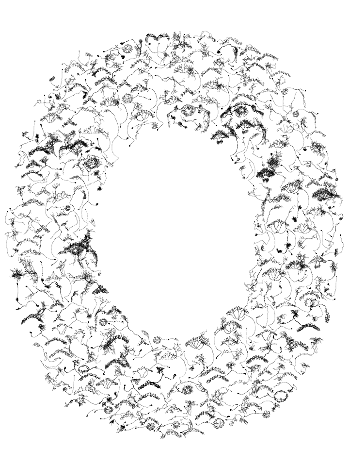
# ### Packing into a shape: `mask`
#
# `mask` confines the neurons to an outline. It takes a bool array covering the page - `True` where neurons
# are allowed, row `0` at the *bottom* - which is resampled to the packing grid, so its resolution does not
# have to match anything:

# A ring: neurons allowed between 45% and 98% of the way out
h, w = 800, 600
yy, xx = np.mgrid[0:h, 0:w]
r = np.hypot((xx - w / 2) / (w / 2), (yy - h / 2) / (h / 2))
mask = (r < 0.98) & (r > 0.45)

fig, ax, placed = navis.plot_collage(
    nl, layout="dense", mask=mask, page_size=(6, 8), radius="lw", color="k"
)

# %%
# ![mask](../../../_static/collage_tut/08_mask.png)
#
# !!! note "Masks always pack by occupancy"
#     Bounding boxes cannot follow an arbitrary outline, so a `mask` implies `occupancy=True` - there is no
#     box layout to start the search from, which makes it a bit slower than the plain dense layout. The
#     neurons are laid down from the middle of the shape outwards; filling bottom-up, as the unmasked
#     layouts do, would leave the top of the shape bare.
#
# `mask` also takes a *picture* of the shape - a file path or the pixels - which is scaled onto the page
# with dark counting as the shape:
#
# ```python
# fig, ax, placed = navis.plot_collage(nl, layout="dense", mask="my_silhouette.png")
# ```
#
# ## Colors
#
# `color` is either one color for all neurons or **one per neuron**, in the order of `x`. Colors follow
# their neurons through whatever the layout does with them - `sort` reorders them, `drop_dangling` and a
# dropped `backfill` neuron take their color along.
#
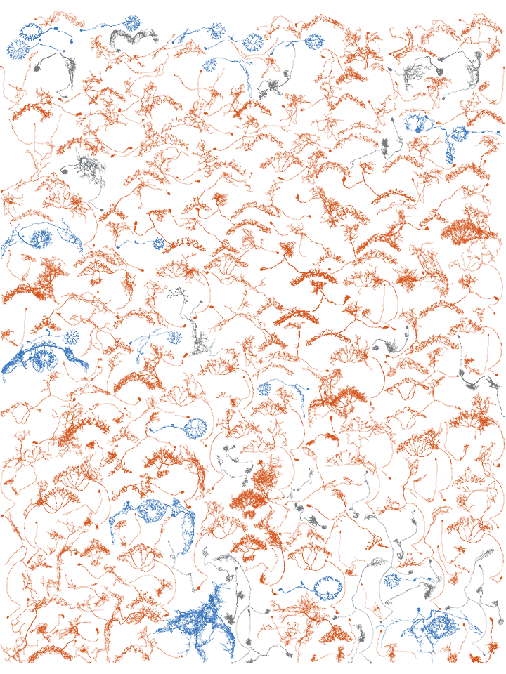
# Let's color our CX neurons by the structure their name points at:

PALETTE = {"FB": (0.85, 0.33, 0.10), "EB": (0.20, 0.45, 0.75), "other": (0.45, 0.45, 0.45)}
GROUPS = {"FB": ("FB", "FC", "FS", "FR", "hDelta", "vDelta"), "EB": ("ER", "ExR", "EL", "EP")}


def group(name):
    for grp, prefixes in GROUPS.items():
        if name.startswith(prefixes):
            return grp
    return "other"


colors = [PALETTE[group(n.name)] for n in nl]

fig, ax, placed = navis.plot_collage(
    nl, layout="dense", occupancy=True, page_size=(6, 8), radius="lw", color=colors
)

# %%
# ![colors](../../../_static/collage_tut/09_colors.png)
#
# !!! tip "`color_by` works too"
#     Anything `plot_collage` does not recognise is handed straight to [`navis.plot2d`][], including
#     `color_by`/`palette` - see the [coloring tutorial](../1a_plotting_general/tutorial_plotting_01_colors).
#     The placed copies keep the properties of the originals, so coloring by a node column or a neuron
#     property works exactly as it does anywhere else.
#
# ## Re-using a layout
#
# The third return value, `placed`, holds the scaled and moved copies in the order they were plotted.
# Hand them back in as `placed=` and the layout is skipped entirely - the same page, re-drawn:

# Re-plot the page we just packed, in a different color
fig, ax, _ = navis.plot_collage(placed=placed, page_size=(6, 8), radius="lw", color="k")

# %%
# !!! warning "`view` and `page_size` still apply"
#     Every *layout* parameter is ignored when you pass `placed`, but `view` and `page_size` are not - they
#     have to match the ones the neurons were laid out with, or the page will not line up.
#
# That is worth knowing because packing 200 arbors by occupancy takes a few seconds, and you will rarely
# get the colors right first time. It is also how you swap the renderer without re-packing:
#
# | `backend` | How it draws | Trade-off |
# |-----------|--------------|-----------|
# | `"matplotlib"` (default) | every neuron as vector paths via [`navis.plot2d`][] | scalable and editable afterwards, but the file grows with the amount of cable on the page |
# | `"octarine"` | renders the page offscreen via [`navis.plot3d`][]`(snapshot=True)` and places the image | fixed size no matter how dense the page (160 neurons: 8.9 MB of SVG against 1.0 MB), and shades meshes the way the interactive viewer does |
#
# ```python
# fig, ax, _ = navis.plot_collage(placed=placed, backend="octarine", page_size=(6, 8))
# ```
#
# Either way you get a matplotlib figure back with the neurons in their own coordinates, so a page looks
# the same whichever one drew it - and annotations, scale bars or an inset land in the same place.
#
# ## Where to next
#
# <div class="grid cards" markdown>
#
# -   :material-image-outline: **2D plotting**
#
#     Everything you can hand through `**kwargs`: radius, tapering, halos and depth sorting.
#
#     [:octicons-arrow-right-24: Skeletons](../1b_plotting_2d/tutorial_plotting_2d_00_skeletons) ·
#     [Meshes](../1b_plotting_2d/tutorial_plotting_2d_01_meshes)
#
# -   :material-palette-outline: **Coloring**
#
#     Palettes, `color_by` and depth coloring - the same in every backend.
#
#     [:octicons-arrow-right-24: Colors](../1a_plotting_general/tutorial_plotting_01_colors)
#
# </div>
#
# *[CX]: Central complex - a set of midline neuropils in the insect brain.
# *[SVG]: Scalable Vector Graphics - a resolution-independent, text-based image format.

# %%

# mkdocs_gallery_thumbnail_path = '_static/collage_tut/00_thumbnail.png'